MAT1001 Differential Calculus: Lecture Notes
Chapter 6 Numerical Methods
6.1 Solving equations numerically
It frequently happens that when confronted with a problem you end up with a mathematical problem or expression that cannot be evaluated analytically. This may be a differential equation that we cannot solve, an integral that has no closed form solution, or even an
algebraic equation which does not yield an explicit solution. This is where we have to turn to computer packages or follow a numerical method. Nowadays many computer programs can implement these approaches as standard. However, it is a good idea to understand
how to implement a few of these approaches by hand as you may end up writing one of your own at some stage.
Chapter 27 of [Riley et al., 2006] contains a lot of information about this topic and is a good place to go for more details than we will discuss here.
Before moving on to numerical differentiation and integration we will first discuss how to solve algebraic equations numerically. This is all about finding the real roots of an equation \(f(x)=0\). This equation can either be algebraic, with \(f(x)\) being a polynomial, or
transcendental, if \(f(x)\) includes trig, log, or exponential terms. We will be using iterative schemes to solve the equations, where we make successive approximations to the true solution, which converge to the true solution. For a method to be successful we need both
that the approximations converge to the true solution, and also that we only have a finite number of solutions.
It is important to note that different iteration methods will be better at solving certain kinds of problems, in practice some combination of methods is likely to be used. We will see four methods, Rearrangement, Linear interpolation, and Bisection, before discussing Newton’s method, which is the most important method to know in this module.
Rearrangement
To explain what we mean by an iterative scheme it is useful to consider the first example method, recasting our equation \(f(x)=0\) as
\(\seteqnumber{0}{6.}{0}\)\begin{equation*} x=\phi (x), \end{equation*}
for some slowly varying function \(\phi (x)\). Our iteration scheme starts from a guess, \(x_{0}\) which will not solve \(f(x_{0})=0\) but should be picked so that it is close to zero1. We then have that \(x_{1}=\phi (x_{0})\) and can keep repeating this
process, i.e. \(x_{n+1}=\phi (x_{n})\). The solution we are looking for will be a value of \(x\) that is left unchanged by applying \(\phi \).
The different methods are different ways of building \(\phi (x)\) so that we can start the iteration scheme.
As an example of how to use the rearrangement iteration consider
\(\seteqnumber{0}{6.}{0}\)\begin{equation} f(x)=x^{5}-3x^3+2x-4=0. \label {eq: equation for iterating} \end{equation}

By rearranging this equation we have that
\(\seteqnumber{0}{6.}{1}\)\begin{equation*} x=\left (3x^{3}-2x+4\right )^{\frac {1}{5}}. \end{equation*}
From the plot we in fig. 6.1 we see that the root is between \(x=1.5\) and \(x=2\) and to see how the method works we will not attempt to start from that close to the true root. Here we take \(x_{0}=1.8\) and then iterate using
\(\seteqnumber{0}{6.}{1}\)\begin{equation*} x_{n+1}=\left (3x_{n}^{3}-2x_{n}+4\right )^{\frac {1}{5}}. \end{equation*}
The successive values of \(x_{n}\) and \(f(x_{n})\) are shown in table 6.1 and they are closing in on
\(\seteqnumber{0}{6.}{1}\)\begin{equation} x=1.757632748, \label {eq: precise root} \end{equation}
which is the value of the root to \(9\) decimal places. We see from the table that once we got to \(x_{5}\) we were only differing from the precise answer in the third decimal places, so are within two parts in \(10^{3}\). We can also see that lots of iterations are needed
to get an accurate answer. The precise number will depend on the specific problem.
| \(n\) | \(x_{n}\) | \(f(x_{n})\) |
| \(0\) | \(1.8\) | \(0.99968\) |
| \(1\) | \(1.7805378\) | \(0.52247969\) |
| \(2\) | \(1.7700175\) | \(0.27736234\) |
| \(3\) | \(1.7643295\) | \(0.14849136\) |
| \(4\) | \(1.761254\) | \(0.07986324\) |
| \(5\) | \(1.7595909\) | \(0.043059716\) |
| \(12\) | \(1.75765592\) | \(0.00058017842\) |
| \(18\) | \(1.7576331\) | \(7.8434818\times 10^{-6}\) |
1 It is useful to plot or roughly sketch the function \(f(x)\) as then it can be easier to pick a starting point.
-
Exercise 6.1. Implement this iteration method numerically for eq. (6.1) using a programming language or computer program of your choice. I would suggest trying Python or Matlab, but you can use whatever you feel most comfortable with.
Linear interpolation
The next method to look at is linear interpolation. The idea here is to pick two points \(A_{1},B_{1}\) on the graph \(y=f(x)\) that lie on either side of the root, i.e. so that \(f(A_{1})\) and \(f(B_{1})\) have opposite signs. We can then think about the
straight line2 joining these points \((A_{1},f(A_{1}))\) to \((B_{1},f(B_{1}))\). An example of this is shown in fig. 6.2 where \(A_{1}=1.5\) and \(B_{1}=1.8\).
The intersection of this straight line with the \(x\)-axis is given by
\(\seteqnumber{0}{6.}{2}\)\begin{equation*} x_{1}=\frac {A_{1}f(B_{1})-B_{1}f(A_{1})}{f(B_{1})-f(A_{1})}, \end{equation*}
We then replace \(A_{1}\) or \(B_{1}\) by \(x_{1}\), find the point on the curve corresponding to \(x=x_{1}\) and then iterate this process using the interpolation formula
\(\seteqnumber{0}{6.}{2}\)\begin{equation} x_{n}=\frac {A_{n}f(B_{n})-B_{n}f(A_{n})}{f(B_{n})-f(A_{n})}. \label {eq: linear interpolation formula} \end{equation}

With each iteration the chord will become shorter and the end points will move until the value of \(x_{n}\) converges to the precise value of the root. The first few steps of this interpolation starting from \(A_{1}=1.5\) and \(B_{1}=1.8\) are shown in table 6.2.
| \(n\) | \(A_{n}\) | \(f(A_{n})\) | \(B_{n}\) | \(f(B_{n})\) | \(x_{n}\) | \(f(x_{n})\) |
| \(1\) | \(1.5\) | \(-3.5315\) | \(1.8\) | \(0.99968\) | \(1.50003\) | \(-3.5310\) |
| \(2\) | \(1.50003\) | \(-3.5310\) | \(1.8\) | \(0.99968\) | \(1.50006\) | \(-3.53082\) |
| \(3\) | ||||||
| \(4\) | ||||||
| \(5\) |
We can see from this example that the linear interpolation method is much slower than rearrangement method, this will not always be true, but is your first hint that you should play around with several approaches before settling on the one that works the best. If you are writing code for these problems, then it is a good idea to have code that can implement any of the iteration schemes that we are discussing here.
Bisection method
Another method for finding roots is the Bisection method. Consider a root \(a\) of a function \(f(x)\). The idea here is to guess two points, one on either side of the root \(a\), and then keep shrinking the size of the interval until we have an estimate of the value of the
root. Since the function is zero at the root, we can check that we have actually picked points on either side of the root by checking that the function has different signs on either side of the interval.
-
Example 6.2. Consider the function \(f(x)=x^{4}+2x-2\), we start by guessing that the root is contained in the interval \([1/2, 1]\). We can check this by computing that \(f(1/2)=-0.9375\) while \(f(1)=1\). Since the function changes sign across the interval, we know that it has a zero in the interval. We call the left end of teh interval \(a_{0}\) and the right end \(b_{0}\), and for each step of refining the interval we will have an \(a_{r}\) and a \(b_{r}\). To narrow down the position of the root we find the mid point of the interval and evaluate the function there:
\(\seteqnumber{0}{6.}{3}\)\begin{equation*} c_{1}=\frac {a_{1}+b_{1}}{2}=\frac {1/2 +1}{2}=\frac {3}{4}=0.75. \end{equation*}
and \(f(0.75)=-0.1836\). Since this is still negative we then know that the root lies in the interval \([0.75,1]\) and again we can find the new mid point:
\(\seteqnumber{0}{6.}{3}\)\begin{equation*} c_{2}=\frac {a_{2}+b_{2}}{2}=\frac {0.75 +1}{2}=0.875,. \end{equation*}
with \(f(0.875)=0.3362\). Since this is positive we can again restrict the interval to \([0.75,0.875]\). We can keep repeating this until we get the desired precision. Though it is much easier to do this in a table, as seen in table 6.3
Table 6.3: Successive approximations to the root of \(x^{4}+2x-2\) using the bisection method.\(r\) \(a_{r}\) sign of \(f(a_{r})\) \(b_{r}\) sign of \(f(b_{r})\) \(c_{r}\) sign of \(f(c_{r})\) \(1\) \(0.500000\) \(-\) \(1.000000\) \(+\) \(0.750000\) \(-\) \(2\) \(0.750000\) \(-\) \(1.000000\) \(+\) \(0.875000\) \(+\) \(3\) \(0.750000\) \(-\) \(0.875000\) \(+\) \(0.812500\) \(+\) \(4\) \(0.750000\) \(-\) \(0.812500\) \(+\) \(0.781250\) \(-\) \(5\) \(0.781250\) \(-\) \(0.812500\) \(+\) \(0.796875\) \(-\) \(6\) \(0.796875\) \(-\) \(0.812500\) \(+\) \(0.804688\) \(+\) \(7\) \(0.796875\) \(-\) \(0.804688\) \(+\) \(0.800781\) \(+\) \(8\) \(0.796875\) \(-\) \(0.800781\) \(+\) \(0.798828\) \(+\) If we want an answer to two decimal places we find that the root is at \(x=0.80\). If we kept going we would find that to four decimal places the root is at \(x=0.7976\).
Newton’s method
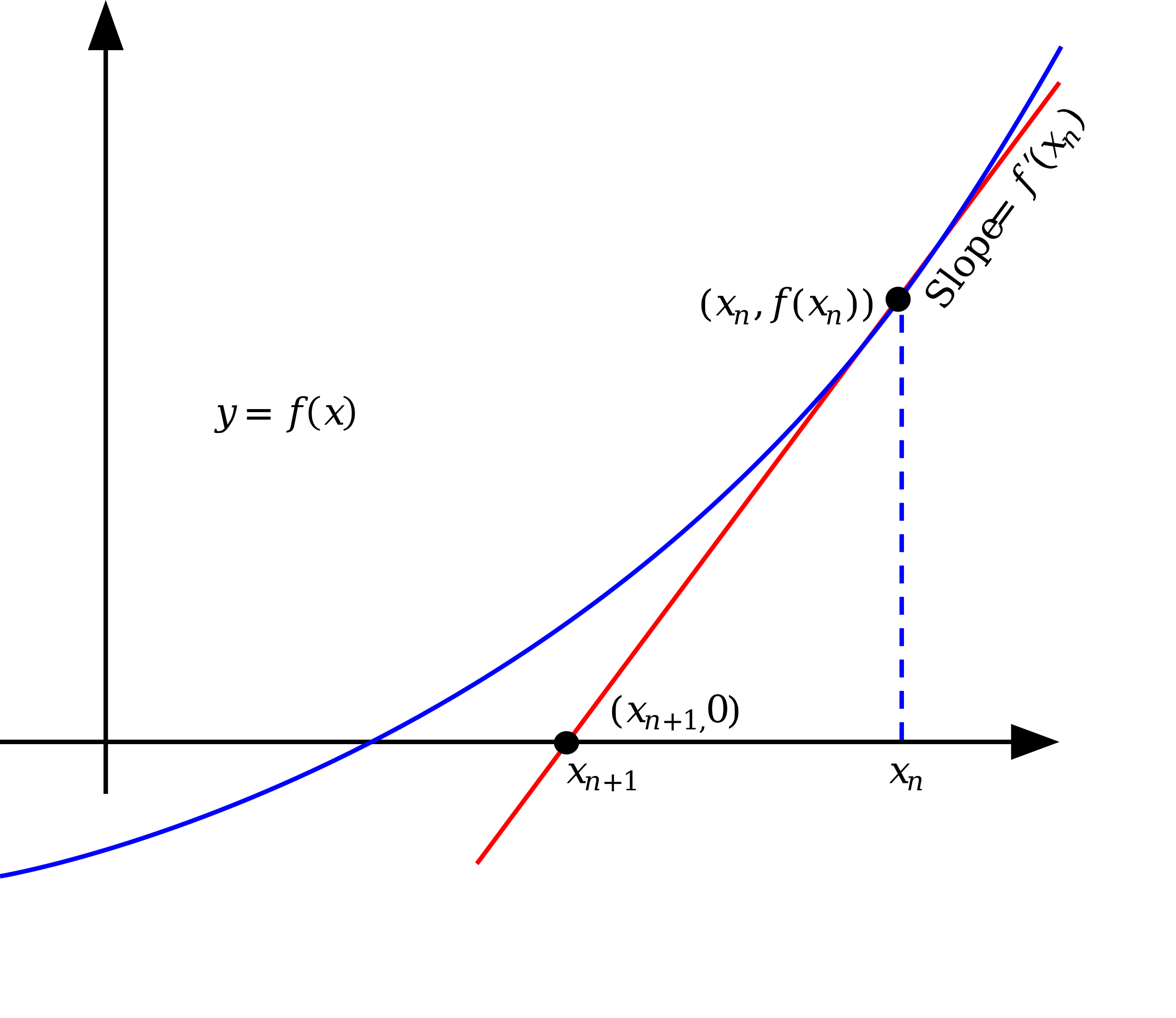
The main numerical method that is needed in this module is Newton’s method, sometimes called the Newton-Raphson method. Newton’s method finds the root by constructing the tangent to a curve through the initial point \(x_{0}\), and then
taking the next point \(x_{1}\) to be where the tangent line intersects the \(x\)-axis.
| \(n\) | \(x_{n}\) | \(f(x_{n})\) |
| \(0\) | \(1.8\) | \(0.99968\) |
| \(1\) | \(1.760530638\) | \(0.06382986248\) |
| \(2\) | \(1.757647406\) | \(0.00032122929\) |
| \(3\) | \(1.757632748\) | \(8.267167839\times 10^{-9}\) |
| \(4\) | \(1.757632748\) | \(-8.881784197\times 10^{-16}\) |
| \(5\) | \(1.757632748\) | \(-8.881784197\times 10^{-16}\) |
In other words we start from a guess, \(x_{0}\), then construct the tangent line
\(\seteqnumber{0}{6.}{3}\)\begin{equation*} y(x)=\left (x-x_{0}\right )f'(x_{0})+f(x_{0}). \end{equation*}
Once we have the tangent we find the value of \(x\) such that \(y(x)=0\) and call this \(x_{1}\). Doing this for a general point in the iteration \(x_{n}\) the iteration scheme is
\(\seteqnumber{0}{6.}{3}\)\begin{equation} x_{n+1}=x_{n}-\frac {f(x_{n})}{f'(x_{n})}. \label {eq: Newton iteration scheme} \end{equation}
An important observation here is that if the points \(x_{n}\) get close to a critical point of \(f(x)\) then the scheme will break down as then \(f'(x_{n})\) will be approaching zero. This means that we need to be very careful about picking our starting point, if we
pick one that is on the opposite side of a critical point from a root then we may not be able to get to the root. Figure 6.3 shows what the first step in Newton’s method looks like graphically.
For the specific equation in eq. (6.1) we have that
\(\seteqnumber{0}{6.}{4}\)\begin{equation} x_{n+1}=x_{n}-\frac {x_{n}^{5}-3x_{n}^3+2x_{n}-4}{5x_{n}^{4}-9x_{n}^{2}+2}. \end{equation}
Starting from \(x_{0}=1.8\) we get the sequence in table 6.4. This iteration scheme converges to the precise answer of eq. (6.2) much quicker than the other methods.
Newton’s method is the approach that you need to be able to use during this module so we will treat a couple more examples using it. There are a couple more examples on [Dawkins, 2025b] if you want to see more.
-
Example 6.4. Use Newton’s method to determine an approximation to the solution to \(\sin {x} = -x\) that lie in the interval \([-1,1]\). Find the approximation to \(6\) decimal places.
First we need to pick a starting point \(x_{0}\). Here we will take \(x_{0}=0.5\), you can get an idea of what value to pick by plotting the function. For this example we have that
\(\seteqnumber{0}{6.}{5}\)\begin{equation} f(x)=\sin (x)+x=0, \label {eq: sin +x roots} \end{equation}
so the iteration equation for Newton’s method eq. (6.4) becomes
\(\seteqnumber{0}{6.}{6}\)\begin{equation*} x_{n+1}=x_{n}-\frac {\sin {x_{n}}+x_{n}}{\cos {x_{n}}+1}. \end{equation*}
The first approximation is then
\(\seteqnumber{0}{6.}{6}\)\begin{equation*} x_{1}=\frac {1}{2}-\frac {\sin {\frac {1}{2}}+\frac {1}{2}}{\cos {\frac {1}{2}}+1}=-0.0216418 \end{equation*}
Table 6.5: Successive approximations to the root of eq. (6.6) using Newton’s method.\(n\) \(x_{n}\) \(f(x_{n})\) \(0\) \(0.5\) \(0.979426\) \(1\) \(-0.021642\) \(-0.043282\) \(2\) \(2\times 10^{-6}\) \(3.\times 10^{-6}\) \(3\) \(0\) \(0\) The further iteration steps are shown in table 6.5, and we see that to 6 decimal places, it only takes \(4\) iterative steps to find that the root is at \(x=0\). If we did any more steps we would see that these remain at \(x=0\).
Now we can consider one of the examples from [Dawkins, 2025b] which shows when Newton’s method does not work.
-
Example 6.5. Starting from \(x_{0}=1\) we will apply Newton’s method to \(\sqrt [3]{x}\).
Intuitively it is clear that the root is \(x=0\). However, Newton’s method will not find this root. For this example eq. (6.4) becomes
\(\seteqnumber{0}{6.}{6}\)\begin{equation*} x_{n+1}=x_{n}-\frac {\sqrt [3]{x}}{\frac {1}{3}x^{-\frac {2}{3}}}=x_{n}-3x_{n}=-2x_{n}. \end{equation*}
This already tells us that instead of converging to \(x=0\), Newton’s method will diverge with \(x_{1}=-2\), \(x_{2}=4\), \(x_{3}=-8\), \(x_{4}=16\), …. This is the opposite of what we want. Fortunately, it became obvious quite quickly that the method was not working and we did not have to waste much time before discovering that we needed to used a different model.
Secant method
A variant of Newton’s method is the Secant method, where we start with two estimates of the root, \(x_{0}\) and \(x_{1}\) and estimate the derivative as being the Newton quotient
\(\seteqnumber{0}{6.}{6}\)\begin{equation*} Q(x_{0},x_{1})=\frac {f(x_{1})-f(x_{1})}{x_{1}-x_{0}}, \end{equation*}
so that
\(\seteqnumber{0}{6.}{6}\)\begin{equation*} x_{2}=x_{1}-\frac {f(x_{1})}{Q(x_{0},x_{1})}=x_{1}-\frac {f(x_{1})}{\frac {f(x_{1})-f(x_{1})}{x_{1}-x_{0}}}. \end{equation*}
This means that the iteration scheme is given by
\(\seteqnumber{0}{6.}{6}\)\begin{equation} x_{n+1}=x_{n}-\frac {f(x_{n})}{Q(x_{n-1},x_{n})}=x_{n}-\frac {f(x_{n})}{\frac {f(x_{n})-f(x_{n-1})}{x_{n}-x_{n-1}}} \label {eq: secant method} \end{equation}
Geometrically, the secant method can also be viewed as constructing a line nearby our function and moving to the point where this line cuts the \(x\)-axis. However, this line is no longer a tangent line, but is a secant.
-
\(\seteqnumber{0}{6.}{7}\)
\begin{equation*} f(x)=x^{2}-10, \end{equation*}
and taking \(x_{0}=2\), \(x_{1}=3\) we find \(x_{2}\) using the secant method as follows:
\(\seteqnumber{0}{6.}{7}\)\begin{align*} x_{2}&=x_{1}-\frac {f(x_{1})}{\frac {f(x_{1})-f(x_{0})}{x_{1}-x_{0}}}\\ &=3-\frac {-1}{\frac {-1-(-6)}{3-2}}\\ &=3+\frac {1}{7}\\ &=3.14286. \end{align*} This is an equation that we can solve directly by the rearrangement method since \(f(x)=0\) corresponds to \(x^{2}=10\) so the exact answers are \(x=-\sqrt {10}\simeq -3.16228\) and \(x=\sqrt {10}\simeq 3.16228\). We can see that \(x_{2}\) is already approaching this exact answer.
Convergence and errors
The absolute error of a numerical method is the difference between the true solution \(x\) and the approximate solution \(\xi \), \(\epsilon =\vert x-\xi \vert \). It can be hard to estimate the absolute error unless we already know the exact solution.
We say that an iteration scheme converges when it subsequent iterations do not change the value of \(x_{n}\), at least to the accuracy that we are looking for. Not every method will converge for a given problem, We have already seen that Newton’s method does not converge for the cube root, \(\sqrt [3]{x}\). You will gain experience of which methods works best for which type of of problem. In this module, you will mainly be using Newton’s method so you need to remember that it can fail.
6.2 Approximating functions
Through much of this module we have been discussing functions and how to work with them. Now we will look at a method for approximating functions using polynomials. This is one of the reasons that we spent so long discussing polynomials at the start. If we can
understand polynomials then we can get a good idea of how many functions behave.
In essence this function is all about fitting data points, or establishing if there is a relationship or trend between known data. We are not framing it like this here but if you go on to take any statistics or data analysis modules then the approximation ideas here will prove useful to you.
If we have time, in chapter 8 we will discuss the continuous analogue of this which goes by the name of the Taylor or Maclaurin series. However, to understand these properly, we need to know how to calculate multiple derivative, which is just at the edge of what is included in this module. In this section we will be doing this using two discrete methods, one known as the Newton interpolating polynomial, or Newton’s divided difference method, and the other Lagrange’s method.
Newton’s method
The idea is that idea is that given some values of a function, we can find a polynomial which passes through them. The example given in [Lissamen and West, 2004] is to consider the growth rate per year for a group of young people. The results are given in table 6.6 and can be plotted as five points on a graph. The question asked, and answered, in [Lissamen and West, 2004] is can a formula be found which fits all of these points. The formula given in [Lissamen and West, 2004] is
\(\seteqnumber{0}{6.}{7}\)\begin{equation*} f(x)=4.13984375+3.34791667x-0.91315104x^{2}+0.08177083x^{3}-0.00232747x^{4}. \end{equation*}
The intuition behind this is that we first guess that the function has the form of a straight line \(f(x)=mx+c\), notice that this does not fit the data, then add higher order monomials such as \(x^{2},x^{3},x^{4}\) with appropriate sized coefficients until we get the
correct shape and the curve passes through, or close to, the points.
By the end of this section you will know how to calculate the approximate function which fits the given data.

Following [Lissamen and West, 2004], we will use the notation in table 6.7. We start our labelling from the left most point and moving rightwards until we get to the
last point. Here we are taking \(x\) values that have a constant spacing which we denote by \(h\)3.
One approach to finding the polynomial is via a finite difference table. This is a means of keeping track of the points, the values of the function at the points, the differences between the values of the function at neighbouring points, the differences between the differences,
and so on.
As usual we take \(\Delta \) to mean the change in some quantity. Here it is technically being used to denote the forward difference operator,
\(\seteqnumber{0}{6.}{7}\)\begin{equation} \Delta f_{0}=f_{1}-f_{0}, \quad \Delta f_{1}=f_{2}-f_{1}, \quad \dots , \Delta f_{n-1}=f_{n}-f_{n-1}. \label {eq: forward differences} \end{equation}
This is called the forward difference because it is defined as \(f_{1}-f_{2}\), e.g we subtract the value of the function at the point on the left from the value at the point on the left. There is a corresponding backward difference operator coming from
considering \(f_{0}-f_{1}\). We will not consider backwards differences here, but you can come up with an alternative method using them. If you go into numerical analysis, or solving real world problems by writing computer programmes then you will need to be
familiar with both methods.
The differences between differences are then denoted
\(\seteqnumber{0}{6.}{8}\)\begin{equation} \Delta ^{2}f_{0}=\Delta f_{1}-\Delta f_{0}, \quad \Delta ^{2}f_{1}=\Delta f_{2}-\Delta f_{1}, \dots . \end{equation}
If we wanted to we can keep going with differences of differences of differences etc. How far you go will depend on the specific problem, as well as how precise you want your approximation to be.
A convenient way to keep track of everything is to put it all in a table as in table 6.8 which has four points and works up to third order differences \(\Delta ^{3}f_{i}\). If we wanted to include more differences then we would need to add more columns.
| \(x_{i}\) | \(f_{i}\) | \(\Delta f_{i}\) | \(\Delta ^{2} f_{i}\) | \(\Delta ^{3}f_{i}\) |
| \(x_{0}\) | \(f_{1}\) | |||
| \(\Delta f_{0}=f_{1}-f_{0}\) | ||||
| \(x_{1}\) | \(f_{1}\) | \(\Delta ^{2}f_{0}=\Delta f_{1}-\Delta f_{0} \) | ||
| \(\Delta f_{1}=f_{2}-f_{1}\) | \(\Delta ^{3}f_{0}=\Delta ^{2}f_{1}-\Delta ^{2}f_{0}\) | |||
| \(x_{2}\) | \(f_{2}\) | \(\Delta ^{2}f_{1}=\Delta f_{2}-\Delta f_{1}\) | ||
| \(\Delta f_{2}=f_{3}-f_{2}\) | ||||
| \(x_{3}\) | \(f_{3}\) |
3 If this seems suggestive of our notation when doing differentiation from first principles, that is on purpose. The separation between points is precisely what we want to take to zero to get the derivative.
-
Example 6.8. If we consider the data in table 6.6 and work to fourth order differences we get the table in table 6.9. This finite difference table is what we can use to construct the approximate function.
Table 6.9: A finite difference table with four points working up to the third differences for the data in table 6.6.\(x_{i}\) \(f_{i}\) \(\Delta f_{i}\) \(\Delta ^{2} f_{i}\) \(\Delta ^{3}f_{i}\) \(2\) \(7.8\) \(6-7.8 =-1.8\) \(4\) \(6\) \(0-(-1.8)=1.8\) \(6-6=0\) \(0.5-1.8=-1.3\) \(6\) \(6\) \(0.5-0=0.5\) \(6.5-6=0.5\) \(8\) \(6.5\)
-
Example 6.9. Consider the quadratic function \(f(x)=x^{2}+1\), working up to fourth order differences, this gives the finite difference table in table 6.10. Notice that the third and fourth differences all vanish.
Table 6.10: A finite difference table with four points working up to the fourth order differences for the function \(f(x)=x^{2}+1\).\(x_{i}\) \(f_{i}\) \(\Delta f\) \(\Delta ^{2} f\) \(\Delta ^{3}f\) \(\Delta ^{4}f\) \(0\) \(1\) \(1\) \(1\) \(2\) \(2\) \(3\) \(0\) \(2\) \(5\) \(2\) \(0\) \(5\) \(0\) \(3\) \(10\) \(2\) \(7\) \(4\) \(17\)
It is a general property of polynomials that for a polynomial with highest order term \(x^{n}\), the \(n\)’th differences will be constant and all higher order differences will vanish.
The polynomial built from the finite difference table is known as the interpolating polynomial. This gives the interpolating, or approximating function as
\(\seteqnumber{0}{6.}{9}\)\begin{equation} f(x)=f_{0}+\frac {x-x_{0}}{h}\Delta f_{0}+\frac {(x-x_{0})(x-x_{1})}{2!h^{2}}\Delta ^{2}f_{0}+\frac {(x-x_{0})(x-x_{1})(x-x_{2})}{3!h^{3}}\Delta ^{3}f_{0}+\dots , \label {eq: NIP} \end{equation}
with \(h\) the constant spacing between the \(x\) values.
This may look complicated, but there is a set pattern to the terms, and the sum will terminate, either when all of the \(\Delta ^{a}f_{0}=0\) or because of the number of data points we are given.
When we only have two points this method is called linear interpolation as only the first two terms in eq. (6.10) are non-zero.
-
Example 6.12. Consider the finite difference table in table 6.10. The corresponding Newton interpolating polynomial is found as follows:
-
• \(h=1\),
-
• \(\Delta f_{0}=1\),
-
• \(\Delta ^{2}f=2\),
-
• \(\Delta ^{3}f=0\),
and we know what the \(x_{i}\) are, so we can substitute everything in to find:
\(\seteqnumber{0}{6.}{10}\)\begin{align*} f(x) &= 1+x+\frac {x(x-1)}{2}2\\ &=1+x-x+x^{2}=1+x^{2}. \end{align*} This is the polynomial that we started with which is a good sign.
-
-
Exercise 6.13. Consider the finite difference table in table 6.9, and find the Newton interpolation polynomial for this data.
-
Exercise 6.14. Consider the data in table 6.11 and find the polynomial that fits the data.
Then use your approximation to find the value of \(f(4.3)\).
Note that if all of the differences of a given order are approximately constant then we can sometimes get away with a lower order polynomial approximation, even if the higher order terms do not actually vanish.
Lagrange’s method
There is an alternative method due to Lagrange, where we do not need to start with equally spaced points. The easiest way to understand this method is to start by considering the linear case, then the quadratic case, before giving the general expression. This is also
discussed briefly in [Lissamen and West, 2004].
The linear case of Lagrange’s equation is very similar to eq. (6.3) that we met when discussing linear interpolation as a method of root finding.
Given two points \((a,A)\) and \((b,B)\), the straight line that passes through them is given by
\(\seteqnumber{0}{6.}{10}\)\begin{equation*} f(x)=\frac {A(x-b)}{a-b}+\frac {B(x-a)}{b-a} \end{equation*}
where we need that \(a\neq b\).
If we have three points, \((a,A), (b,B), (c,C)\) then they lie on a quadratic given by
\(\seteqnumber{0}{6.}{10}\)\begin{equation*} f(x)=\frac {A(x-b)(x-c)}{(a-b)(a-c)}+\frac {B(x-c)(x-a)}{(b-c)(b-a)}+\frac {C(x-a)(x-b)}{(c-a)(c-b)}, \end{equation*}
where we now need that \(a,b,c\) are non equal.
This approach can be generalised to a polynomial going through \(n\) points. This will be a polynomial of degree \(n-1\) for \(n\) points.
6.3 Numerical integration
This section needs more images added. There are graphs for the mid point rule case but not for the trapezium rule case. These will be added soon.
We now turn to numerical methods of integration. We have already carried out some numerical integration when we discussed definite integrals and the relationship between integrals and sums. In fact the first method we will use to carry out numerical integration, the
midpoint rule, is one we have already seen. We will also discuss two other related rules that estimate the area under a graph, the trapezium rule and Simpson’s rule. These are not independent methods, and Simpson’s rule is actually a
weighted average of the mid point and trapezium rule which improves the accuracy.
In practice, when you ask a computer to carry out a definite integration, unless you use a symbolic computation method in Maple, Mathematica, or similar, the computer will be implementing one of these rules. This means that by understanding how they work and how to implement them by hand, you will be able to code up your own numerical integrator. I recommend this as a challenge to an keen students who want to make practical use of what you are learning in this module and I will put an exercise at the end of each section suggesting that you do this for each of the rules.
Midpoint rule
The mid point rule is the approximation approach that we met in chapter 4 when approximating the area under the curve for the function \(f(x)=x^{2}+1\). Let’s recap it here.
Consider the figure in fig. 6.5, as we saw earlier we will be approximating the area between the curve and the \(x\)-axis, using rectangles of width \(\Delta x\) and height \(\Delta y\).

As before, w e do this by splitting up the interval, \([0,2]\) in this case, into \(n\) subintervals. This will give us an approximation of the area which will improve the more sub integrals we take, in other words the larger that \(n\) is. The width of a subinterval is then
\(\seteqnumber{0}{6.}{10}\)\begin{equation*} \Delta x=\frac {2-0}{n}=\frac {2}{n}. \end{equation*}
In general it will be \(\Delta x=(b-a)/n\), when the interval is \([a,b]\).
Before we said that we could pick the height of the intervals to be any value the function takes within the sub interval. As the numerical approach that we are following is called the midpoint rule, unsurprisingly, we take the height to be the value of the function at the midpoint of the subinterval. Recall that for an interval \([a,b]\) the midpoint is \(c=(a+b)/2\). This method is shown in ??.

As we are taking four subintervals they are
\(\seteqnumber{0}{6.}{10}\)\begin{equation*} \left [0,\frac {1}{2}\right ], \quad \left [\frac {1}{2},1\right ], \quad \left [1,\frac {3}{2}\right ], \quad \left [\frac {3}{2},2\right ], \end{equation*}
which all have width \(\Delta x=1/2\). The heights are
\(\seteqnumber{0}{6.}{10}\)\begin{equation*} f\left (\frac {1}{4}\right )=\frac {17}{16}, \quad f\left (\frac {3}{4}\right )=\frac {25}{16}, \quad f\left (\frac {5}{4}\right )=\frac {41}{16}, f\left (\frac {7}{4}\right )=\frac {65}{16}. \end{equation*}
The area of each rectangle is then
\(\seteqnumber{0}{6.}{10}\)\begin{align*} A_{1}&=\Delta x\times f\left (\frac {1}{4}\right )=\frac {1}{2}\times \frac {17}{16}=\frac {17}{32},\\ A_{2}&=\Delta x\times f\left (\frac {3}{4}\right )=\frac {1}{2}\times \frac {25}{16}=\frac {25}{32},\\ A_{3}&=\Delta x\times f\left (\frac {5}{4}\right )=\frac {1}{2}\times \frac {41}{16}=\frac {41}{32},\\ A_{4}&=\Delta x\times f\left (\frac {7}{4}\right )=\frac {1}{2}\times \frac {65}{16}=\frac {65}{32}. \end{align*}
The total area, \(A_{m}\) since we are using the midpoint rule, is thus
\(\seteqnumber{0}{6.}{10}\)\begin{equation*} A_{m}=A_{1}+A_{2}+A_{3}+A_{4}=\frac {17}{32}+\frac {25}{32}+\frac {41}{32}+\frac {65}{32}=\frac {148}{32}=\frac {37}{8}\simeq 4.625. \end{equation*}
This was a result that we quoted in chapter 4, but did not give all the details for. We also commented on the fact that this was pretty close to the true value of \(A=14/3=4.67\) found by carrying out the definite
integral.
This shows that we do not always need to use that many sub intervals to get a decent estimate of the integral using the midpoint rule.
We have given one example here, and you have checked at least one more on the problem sheets. However, this idea is general.
Given a function \(f(x)\) and an interval \([a,b]\) you should use the following steps:
-
• pick a number of sub intervals, or use the number given in the question, \(n\), and split your interval into \(n\) sub intervals \([a_{0},a_{1}], [a_{1},a_{2}], \dots [a_{n-1},a_{n}]\), of fixed width \(\Delta x =(b-a)/n\).
-
• find the mid point of each sub interval \(c_{i}=(a_{i}-a_{i-1})/2\) and take the height of the rectangle to be the value of the function at this point, \(\Delta y_{i}=f(c_{i})\).
-
• Calculate the area of each of the rectangles as \(A_{i}=\Delta x \times \Delta y_{i}\).
-
• Sum up all of the areas of the rectangles and get your estimate of the total area
\(\seteqnumber{0}{6.}{10}\)\begin{equation*} A_{m}=A_{1}+\dots A_{n}=\sum _{i=1}^{n}A_{i}. \end{equation*}
and use this as your approximation to the definite integral.
In essence we are treating the problem the opposite way round to in chapter 4, where we used this approximate picture and discussed how this became the definite integral in the limit of an infinite number of very
thin rectangles. Here we are saying that we can use a finite number of rectangles to estimate the definite integral.
Note that in many of the cases you are asked about here you can also compute the integrals directly. This enables you to check how close your answer is to the true answer. The real power of this method is that you can approximate the value of integrals that cannot be calculated directly. or which are very hard to calculate directly.
-
Exercise 6.18. Consider the function \(f(x)=x^{3}+x^{2}-x-1\) on the interval \([-1,1]\). Take \(n=6\) and use the midpoint rule to approximate the definite integral
\(\seteqnumber{0}{6.}{10}\)\begin{equation*} I=\int _{-1}^{1}\left (x^{3}+x^{2}-x-1\right )\ud x. \end{equation*}
How does this compare to calculating the definite integral directly?
Trapezium rule
The next rule is known as the trapezium rule. It is very similar to the midpoint rule in that we are approximating the area under the curve using shapes that we know how to calculate the area of. However, here we use trapezia instead of rectangles.
A trapezium is like a rectangle glued onto a triangle, in general it is a four sided shape where at least one pair of sides are parallel. So squares and rectangles are examples of trapezia.
Consider a function \(f(x)\) on the interval \([a,b]\). If the length of the left edge of the trapezium is \(f(a)\) and the length of the right edge is \(f(a+\Delta x)\), while its width is \(\Delta x\), then the area is
\(\seteqnumber{0}{6.}{10}\)\begin{equation*} A_{\text {trap}}=\frac {\Delta x}{2}\left (f(a)+f(a+\Delta x)\right ). \end{equation*}
If we have an interval \([a,b]\) that we split into \(n\) sub intervals of width \(\Delta x=(b-a)/n\) as before, then we use \(n\)-trapezia, one for each sub intervals. The side lengths of the trapezia are:
-
• \(f_{0}=f(a)\) for the left most trapezium,
-
• \(f_{1}=f(a+\Delta x)\) for the right side of the first sub interval and the left side of the second,
-
• \(f_{2}=f(a+2\Delta x)\) for the right side of the second sub interval and the left side of the third, and so on up to
-
• \(f_{n}=f(a+n\Delta x)=f(b)\) for the right side of the \(n\)’th sub interval.
The area of the trapezia are thus
\(\seteqnumber{0}{6.}{10}\)\begin{align*} A_{1}&=\frac {\Delta x}{2}\left (f_{0}+f_{1}\right ),\\ A_{2}&=\frac {\Delta x}{2}\left (f_{1}+f_{2}\right ),\\ \dots &\dots \\ A_{n}&=\frac {\Delta x}{2}\left (f_{n-1}+f_{n}\right ). \end{align*}
Summing these up gives
\(\seteqnumber{0}{6.}{10}\)\begin{equation} \begin{split} A_{T} &=A_{1}+A_{2}+\dots +A_{n}\\ &=\frac {\Delta x}{2}\left (f_{0}+f_{1}\right )+\frac {\Delta x}{2}\left (f_{1}+f_{2}\right )+\dots +\frac {\Delta x}{2}\left (f_{n-1}+f_{n}\right )\\ &=\frac {\Delta x}{2}\left (f_{0}+2\left (f_{1}+f_{2}+\dots +f_{n-1}\right )+f_{n}\right ). \end {split} \label {eq: trapezium rule} \end{equation}
Thus to estimate the integral using the trapezium rule we just need to know the value of the function at the end points of the intervals, and the width of the intervals.
-
Example 6.20. Consider \(f(x)=\cos (x)\) over the interval \([0,\uppi /2]\). In [Lissamen and West, 2004], they discuss this example for \(1,2,4\) and \(8\) sub intervals, here we will just treat the case of \(n=4\), so \(\Delta x= \uppi /8\). The easiest way to keep track of the information we need is in a table of points, the boundaries of the interval, and the value of the function at these points. This table is shown in table 6.12. taking these five values of \(f(x)\) and substituting into eq. (6.11) we get
\(\seteqnumber{0}{6.}{11}\)\begin{align*} A_{T} &=\frac {\Delta x}{2}\left (f_{0}+2\left (f_{1}+f_{2}+f_{3}\right )+f_{4}\right )\\ &=\frac {\uppi }{16}\left (1+2(0.92+\frac {1}{\sqrt {2}}+0.38)+0\right )\\ &=0.98, \end{align*} which is close to the true value of \(1\).
Note that both the trapezium rule and the midpoint rule can be used to find the area under a curve even if we do not know the form of the function.
-
Consider that we are given the data in table 6.13, using just this information we can find
\(\seteqnumber{0}{6.}{11}\)\begin{equation*} \int _{1}^{3}f(x)\ud x, \end{equation*}
without knowing the form of \(f(x)\) using the trapezium rule.
This works as follows. We have \(n=4\) sub intervals defined by the five values of \(x\) we are given. Thus we can use eq. (6.11), and \(\Delta x=(3-1)/4=1/2\) to find
\(\seteqnumber{0}{6.}{11}\)\begin{align*} A_{T} &=\frac {\Delta x}{2}\left (f_{0}+2\left (f_{1}+f_{2}+f_{3}\right )+f_{4}\right )\\ &=\frac {1}{4}\left (0+2\left (0.41+0.69+0.92\right )+1.10\right )\\ &=1.29. \end{align*}
Note that we could use Newton’s divided difference method to find an approximation to this function, but we do not need to do this to calculate the integral.
-
Exercise 6.23. Use the trapezium rule with 4 steps to approximate the definite integral
\(\seteqnumber{0}{6.}{11}\)\begin{equation*} I=\int _{0}^{2}\left (x^{2}+1\right )\ud x \end{equation*}
and compare it to the answer that we got using the mid point rule in chapter 4.
Simpson’s rule
The final numerical method that we will discuss is Simpson’s rule. This is a weighted average of the trapezium rule and the mid point rule. We could actually consider any weighted average of the the two methods to get an approximation to the definite integral. However, if we were analysing the error we would see that there is one particular choice which minimises the error and gets as close as possible to the true value of the integral. This is Simpson’s rule,
\(\seteqnumber{0}{6.}{11}\)\begin{equation} A_{S}=\frac {2A_{m}+A_{T}}{3}. \label {eq: simpsons rule} \end{equation}
Note that here we would use the same number of intervals for both the midpoint rule and the trapezium rule.
-
Example 6.25. Let’s return to one of our favourite examples
\(\seteqnumber{0}{6.}{12}\)\begin{equation*} I=\int _{0}^{\frac {\uppi }{2}}\cos (x)\ud x \end{equation*}
and calculate this for \(n=4\) sub intervals using Simpson’s rule.
The data to calculate this is given in table 6.12, though we need to find the value of the function at the midpoints for the midpoint rule. We already know that \(A_{T}=0.98\) so we just need to find \(A_{m}\). The four mid points and the value of the function at them are:
-
• \(c_{0}=(\uppi /8 +0)/2=\uppi /16\) and \(\cos (c_{0})=0.98\)
-
• \(c_{1}=(\uppi /4 +\uppi /8)/2=3\uppi /16\) and \(\cos (c_{1})=0.83\),
-
• \(c_{2}=(3\uppi /8 +\uppi /4)/2=5\uppi /16\) and \(\cos (c_{2})=0.556\)
-
• \(c_{3}=(\uppi /2 +3\uppi /8)/2=7\uppi /16\) and \(\cos (c_{3})=0.195\)
We thus have that
\(\seteqnumber{0}{6.}{12}\)\begin{align*} A_{m}&=\Delta x\left (f(c_{0})+f(c_{1})+f(c_{2})+f(c_{3})\right )\\ &=\frac {\uppi }{8}\left (0.98+0.83+0.556+0.195\right )\\ &=1.0057. \end{align*}
Simpson’s rule then gives that
\(\seteqnumber{0}{6.}{12}\)\begin{equation*} A_{S}=\frac {2A_{m}+A_{T}}{3}=0.997\simeq 1 \end{equation*}
where we have rounded to two decimal places.
-
6.4 Numerical differentiation
We now turn to numerical approaches to differentiation. We have seen hints of this in the background when discussing other topics, including as far back as when we discussed differentiation from first principles.
A major reason that we need a numerical approach to differentiation is that the definition of differentiation from first principles is very hard to implement on a computer. It is much easier for a computer to understand an approximate method.
Forward difference method
The key idea is to look at the definition of differentiation from first principles in eq. (3.1), and drop the limit part. e.g. we calculate an approximate gradient for points a small difference apart. In other words,
\(\seteqnumber{0}{6.}{12}\)\begin{equation} \frac {\ud f}{\ud x}\simeq \frac {f(x+h)-f(x)}{h}=\frac {\Delta f}{h}, \label {eq: forward difference approx} \end{equation}
for \(h\) a small step between neighbouring points. This is known as the forward difference method, since we are looking at the difference between the function at the point \(x\) and at the point \(x+h\) one step ahead of \(x\). This is shown schematically in
fig. 6.7.

Note that when we are numerically differentiation we will find the value of the derivative of the function at a specific point.
-
Example 6.28. Consider the function \(f(x)=x^{2}\cos (x)\), we can calculate the approximate derivative at \(x=2\) using eq. (6.13) and taking the step size to be \(h=0.1, 0.05, 0.025, 0.0125\). We do this as follows:
-
• \(h=0.1\)
\(\seteqnumber{0}{6.}{13}\)\begin{equation*} \frac {\ud f}{\ud x}(2)\simeq \frac {f(2+0.1)-f(2)}{0.1}=\frac {-2.22637+1.66459}{0.1}=-5.61784, \end{equation*}
-
• \(h=0.05\)
\(\seteqnumber{0}{6.}{13}\)\begin{equation*} \frac {\ud f}{\ud x}(2)\simeq \frac {f(2+0.05)-f(2)}{0.05}=\frac {-1.93766+1.66459}{0.05}=-5.46141, \end{equation*}
-
• \(h=0.025\)
\(\seteqnumber{0}{6.}{13}\)\begin{equation*} \frac {\ud f}{\ud x}(2)\simeq \frac {f(2+0.025)-f(2)}{0.025}=\frac {-1.79914+1.66459}{0.025}=-5.38196, \end{equation*}
\(h=0.0125\)
\(\seteqnumber{0}{6.}{13}\)\begin{equation*} \frac {\ud f}{\ud x}(2)\simeq \frac {f(2+0.0125)-f(2)}{0.0125}=\frac {-1.73136+1.66459}{0.0125}=-5.34196, \end{equation*}
The true value found by calculating the derivative is
\(\seteqnumber{0}{6.}{13}\)\begin{align*} \frac {\ud f}{\ud x}(x)&=2x\cos (x)-x^{2}\sin (x),\\ \frac {\ud f}{\ud x}(2)&=-5.30178, \end{align*} so the approximating is getting closer to this as we take a smaller step size.
-
The forward difference method is not the only approach to approximating the gradient of the tangent line at a point. There are two other popular approaches, the central difference method and the backwards difference method.
Backwards difference method
The backwards difference method is the reverse of the forward difference method. The picture to have in mind, shown in fig. 6.8, is essentially the same as in fig. 6.7. The difference is that now we are comparing the value of the function at point with its value at the point one step earlier. As an equation this is
\(\seteqnumber{0}{6.}{13}\)\begin{equation} \frac {\ud f}{\ud x}\simeq \frac {f(x)-f(x-h)}{h}. \label {eq: backwardsdifference approx} \end{equation}

-
Example 6.30. Similar to in the previous case, consider the function \(f(x)=x^{2}\cos (x)\), we can calculate the approximate derivative at \(x=2\) using the backwards difference method and taking the step size to be \(h=0.1, 0.05, 0.025, 0.0125\). We do this as follows:
-
• \(h=0.1\)
\(\seteqnumber{0}{6.}{14}\)\begin{equation*} \frac {\ud f}{\ud x}(2)\simeq \frac {f(2)-f(2-0.1)}{0.1}=\frac {-1.66459+1.16708}{0.1}=-4.97512, \end{equation*}
-
• \(h=0.05\)
\(\seteqnumber{0}{6.}{14}\)\begin{equation*} \frac {\ud f}{\ud x}(2)\simeq \frac {f(2)-f(2-0.05)}{0.05}=\frac {-1.66459+1.40761}{0.05}=-5.13949, \end{equation*}
-
• \(h=0.025\)
\(\seteqnumber{0}{6.}{14}\)\begin{equation*} \frac {\ud f}{\ud x}(2)\simeq \frac {f(2)-f(2-0.025)}{0.025}=\frac {-1.66459+1.53406}{0.025}=-5.22093, \end{equation*}
\(h=0.0125\)
\(\seteqnumber{0}{6.}{14}\)\begin{equation*} \frac {\ud f}{\ud x}(2)\simeq \frac {f(2)-f(2-0.0125)}{0.0125}=\frac {-1.66459+1.59882}{0.0125}=-5.26143, \end{equation*}
The true value we found before is
\(\seteqnumber{0}{6.}{14}\)\begin{align*} \frac {\ud f}{\ud x}(2)&=-5.30178, \end{align*} so again the approximating is getting closer to this as we take a smaller step size, though this time we are underestimating the gradient and approaching it from below.
-
Central difference method
The central difference method is essentially a combination of the other two methods. In this case we approximate the gradient of the tangent line by using the straight line between the two points \(f(x-h)\) and \(f(x+h)\). In this case we are approximating the derivative by the gradient,
\(\seteqnumber{0}{6.}{14}\)\begin{equation} \frac {\ud f}{\ud x}\simeq \frac {\Delta f}{\Delta x}=\frac {f(x+h)-f(x-h)}{(x+h)-(x+h)}=\frac {f(x+h)-f(x-h)}{2h}. \label {eq: central difference method} \end{equation}
The central difference method is often preferred to the forward and backwards difference method, since it is a higher order method. This means that when we discuss the error we will see that it is quadratic in the small parameter \(h\) while the other methods are linear in \(h\).
-
Example 6.31. Consider \(f(x)=\tan (x)\) and use the central difference method with \(h=0.1, 0.05, 0.025, 0.0125\) to approximate the derivative at \(x=1\). This gives:
-
• \(h=0.1\)
\(\seteqnumber{0}{6.}{15}\)\begin{equation*} \frac {\ud f}{\ud x}(2)\simeq \frac {f(2+0.1)-f(2-0.1)}{0.2}=6.08625, \end{equation*}
-
• \(h=0.05\)
\(\seteqnumber{0}{6.}{15}\)\begin{equation*} \frac {\ud f}{\ud x}(2)\simeq \frac {f(2+0.05)-f(2-0.05)}{0.1}=5.84915, \end{equation*}
-
• \(h=0.025\)
\(\seteqnumber{0}{6.}{15}\)\begin{equation*} \frac {\ud f}{\ud x}(2)\simeq \frac {f(2+0.025)-f(2-0.025)}{0.05}=5.7929, \end{equation*}
\(h=0.0125\)
\(\seteqnumber{0}{6.}{15}\)\begin{equation*} \frac {\ud f}{\ud x}(2)\simeq \frac {f(2+0.0125)-f(2-0.0125)}{0.025}=5.77901, \end{equation*}
The true value of the derivative is \(5.7744\) which our approximations are closing in on.
-
Understanding the error
We briefly mentioned above that the absolute error is the difference between the true value, \(x\), and the value that our approximation returns, \(X\), is given by
\(\seteqnumber{0}{6.}{15}\)\begin{equation} \text {Absolute error}=\vert X-x\vert . \end{equation}
The \(\vert \vert \) mean that this is the absolute value, and of the number within and is always positive. In other words we care about how far away our approximate value is from the true value, but not whether it is greater than or less than the true answer.
The absolute relative error is then
\(\seteqnumber{0}{6.}{16}\)\begin{equation} \text {Absolute relative error}=\left |\frac {X-x}{x}\right |, \end{equation}
and the percentage error is
\(\seteqnumber{0}{6.}{17}\)\begin{equation} \text {Percentage error}=\left |\frac {X-x}{x}\right |\times 100\% \end{equation}
There is a discussion of error and the related concept of convergence of an approximation, i.e. whether the approximation is closing in on the true value and how quickly, in [Lissamen and West, 2004].
-
Example 6.34. Consider the examples of approximating the derivative of \(x^{2}\cos (x)\) using both the backwards and forwards difference method with \(h=0.0125\). The relative and absolute errors are shown in table 6.14.
Table 6.14: A comparison of our approximations to the derivative of \(x^{2}\cos (x)\) at \(x=2\) and the percentage error in each case.Approximate derivative Relative absolute error Percentage error Forward difference \(-5.34196\) \(0.00758 \) \(0.758\% \) Backward difference \(-5.26143\) \(0.00761\) \(0.761\%\)
6.5 Numerical approaches to differential equations
This is a non-examinable section and is not taught every year. It is included in the indicative content of the module but is not assessed in the learning outcomes. Content will be added here at the same time as content is added to chapter 5 since that is the theoretical background for what will be discussed numerically here.