MAT1001 Differential Calculus: Lecture Notes
Chapter 2 Functions
The art of doing mathematics is finding that special case that contains all the germs of generality.
David Hilbert
2.1 What is a function
The concept of a function is essential to understand not just calculus but also computer programming. We can think of a function as being a black box that takes in information, potentially changes it in some way, and then outputs information.

Being more precise, a function is a map between two spaces, the domain (\(X\)), and the codomain (\(Y\)). e.g.
\(\seteqnumber{0}{2.}{0}\)\begin{equation*} f:X\to Y \end{equation*}
and it sends a point \(x\in X\) to a point \(f(x)=y\in Y\). The domain is the space of all allowed inputs, sometimes called the argument of the function. While the codomain is the space that all output of the function have to be in. Many functions cannot reach the whole of the codomain, the subset of outputs that are actually reached by a function are called its image. Functions have the property that they map a point \(x\in X\) to a single point \(y\in Y\),for example:
\(\seteqnumber{0}{2.}{0}\)\begin{equation*} y=f(x)=x^{2}+1, \end{equation*}
is a function since every value of \(x\) gives a single value of \(y\). If we consider what this looks like for a few examples we get:
\(\seteqnumber{0}{2.}{0}\)\begin{align*} x, &\mapsto f(x)=x^{2}+1\\ 0, &\mapsto 0+1=1,\\ \pm 1, &\mapsto 1+1=2,\\ \pm 2, &\mapsto 4+1=5\\ \pm 3, &\mapsto 9+1=10 \end{align*}
However,
\(\seteqnumber{0}{2.}{0}\)\begin{equation*} y^{2}=x+1, \end{equation*}
is not a function since every \(x\) corresponds to two values of \(y\), e.g. if \(x=3\) then \(y^{2}=3+1=4\) and \(y\) can be both \(2\) and \(-2\).
-
Mathematical Diversion 2.1. Note that we some times refer to a square root function \(\sqrt {\phantom {x}}:x\to \sqrt {x}\), even though has more than two outputs for a given input. e.g. \(\sqrt {4}=\pm 2\). It is an example of a multi valued function, and they are important in mathematics, but require care.
Note that when we write \(f(x)\) we are not saying \(f\) times \(x\), but mean that \(f\) is a function of \(x\), e.g. \(f\) takes in a value of \(x\) and returns a number \(y=f(x)\).Sometimes we refer to \(x\) as the argument of the function \(f(x)\).
Throughout this module we will meet several different types of functions so you will need to get familiar with this notation and understand how to evaluate functions. There will be some questions in the tutorial sheet to help you practice this.
A key property of a function is its Roots or zeros, these are the values of \(x\) such that \(f(x)=0\). For linear functions finding the roots is just a matter of rearranging the equation, sometimes referred to as changing the subject. In this module I am assuming
that you have some familiarity with this, if not take a look at the background material in chapter 9 or ask me to point you towards more resources. There will also be some revision questions on this
topic in the first couple of weeks tutorials.
A common type of function where it is, relatively, easy to find the roots is a polynomial. A polynomial is a function given by the sum of powers of a varaiable \(x\), or several variables. There is more information on polynomials in one variable in the polynomials and roots section of chapter 9.
-
Example 2.1. Find all the roots of \(f(x)=9x^{3}-18x^{2}+6x\).
Remember the roots are where \(f(x)=0\) so we are solving \(9x^{3}-18x^{2}+6x=0\). First notice that there is a common factor of \(3x\) in all of the terms so we can factor that out and get
\(\seteqnumber{0}{2.}{0}\)\begin{equation*} 0=9x^{3}-18x^{2}+6x=3x\left (3x^{2}-6x+2\right ). \end{equation*}
This means that either \(x\) is zero or the quadratic expression in brackets, \(3x^{2}-6x+2\), is zero. This means that \(x=0\) is a root of the equation, and there will be two more that we find by solving the quadratic. This can be done by using the quadratic formula:
\(\seteqnumber{0}{2.}{0}\)\begin{align*} x&=\frac {6\pm \sqrt {(-6)^{2}-4(3)(2)}}{2(3)}\\ &=\frac {6\pm \sqrt {12}}{6}\\ &=1\pm \frac {\sqrt {3}}{3}\\ &=1\pm \frac {1}{\sqrt {3}}. \end{align*}
So the three roots of \(f(x)\) are
\(\seteqnumber{0}{2.}{0}\)\begin{equation*} x=0,\quad x=1+\frac {\sqrt {3}}{3},\quad x=1-\frac {\sqrt {3}}{3}. \end{equation*}
If you do not remember how to use the quadratic formula then I suggest that you look at the background material in chapter 9.
-
Mathematical Diversion 2.2. A very useful fact about polynomials, sometimes called the Fundamental Theorem of Algebra, says that a degree \(n\) polynomial has exactly \(n\) roots, counted with multiplicity.
There are a few technicalities here, such as the roots do not have to be real, and will frequently be complex, even if the coefficients of the polynomial are real. Think about the quadratic equation \(x^{2}+1\) which has two imaginary roots at \(x=\pm \ui \).
If this was a course for mathematicians this is where we would spend time talking about the domain and range of a function. How they are defined, and when we need to be careful to avoid dividing by zero. Here, we will not go through this, and I will just remind you that
in your algebraic manipulations you should not divide by any quantity that is zero.
A simple, yet useful, class of functions are the rational functions. There are functions who are the ratio of two polynomials, e.g.
\(\seteqnumber{0}{2.}{0}\)\begin{equation*} f(x)=\frac {4x+10}{x^{2}-2x-15}. \end{equation*}
A useful way to understand a function is draw a graph. In a graph, the domain of the function \(X\) is drawn horizontally and the codomain, \(Y\), is drawn vertically, using Cartesian axes \((x,y)\). The graph consists of the points \((x,y)\) with \(y=f(x)\). In many books \(x\) is called the independent variable and \(y\) the dependent variable. In the tutorials we will discuss how to produce plots using a computer, either using MATLAB, Python, or WolframAlpha. There are also online graphing programs like Desmos and GeoGebra. In these notes most of the graphs are produced using the Tikz package for LaTeX, which is a typesetting and markup language1.
1 If you want to produce professional looking documents which include mathematical formulas then it is worth your time learning how to use LaTeX.
-
Example 2.2. Plot the graph of \(f(x)=2x^{2}-1\).

Note that the equation \(y^{2}=x+1\) also defines a parabola, see fig. 2.3. However if we plot this function the curve is not the graph of a function. You should think about why this is.

-
Example 2.3. The function \(f(x)=\sin (x)\) has the graph shown in fig. 2.4.

When the output of a function is a number, as it will be in this module, we can always add and subtract outputs, as well as multiplying and dividing them. Another, potentially less familiar operation is composition of functions. This is when we take the output from one
function and use this as the input of another function. For example the composition of the functions \(g\) and \(f\) is \(g(f(x))\) and is denoted by \(\left (g\circ f\right )(x)\), and means g acts on the output of \(f(x)\).
-
Example 2.4. Consider the two functions \(f(x)=3x-2\) and \(g(x)=x/3 +2/3\). These satisfy the relationship
\(\seteqnumber{0}{2.}{0}\)\begin{align*} \left (f\circ g\right )(x) &=f\left (g(x)\right )\\ &=f\left (\frac {x}{3}+\frac {2}{3}\right )\\ &=3\left (\frac {x}{3}+\frac {2}{3}\right )-2\\ &=x+2-2=x \end{align*} and
\(\seteqnumber{0}{2.}{0}\)\begin{align*} \left (g\circ f\right )(x)=x. \end{align*}
When we have two functions whose composition leaves \(x\) unchanged, we say that they are Inverse to each other, and \(g\) is the inverse2 of \(f\). As can be seen in Section 1.2 of [Dawkins, 2025b] we can understand this a meaning that if \(f:x\mapsto y\) then \(g:y\mapsto x\), e.g. \(f(-1)=-5\) while \(g(-5)=-1\).
The concept of an inverse function makes intuitive sense. However, if we pretend to be mathematicians and treat this carefully we quickly encounter some problems. For example, what happens if we have a function which sends two different values of \(x\) to the same
value? Then we are unable to know which value we started with, so cannot build an inverse function. For example \(f(x)=x^{2}\) sends both \(x\) and \(-x\) to \(x^{2}\) so we cannot find an inverse that works everywhere, this is why when we first meet the square root
function you often see it as \(\pm \sqrt {\phantom {+}}\).
Mathematicians fix this by introducing the notion of a One-to-one function, sometimes called an injective function. A function is called one-to-one if no two values of \(x\) produce the same value of \(y\), so that
\(\seteqnumber{0}{2.}{0}\)\begin{equation*} f(x_{1})\neq f(x_{2}) \qquad \text { for } x_{1}\neq x_{2}. \end{equation*}
The advantage of one-to-one functions is that we can find inverses for them. If we have two one-to-one functions which satisfy
\(\seteqnumber{0}{2.}{0}\)\begin{equation*} \left (f\circ g\right )(x)=x=\left (g\circ f\right )(x), \end{equation*}
then \(f\) and \(g\) are inverses and we write \(g(x)=f^{-1}(x)\).
2.2 Trigonometric functions
Now that we have discussed functions and how to graph them, we can focus on some specific functions which it is very common to encounter.
From your previous maths experience you have probably come across Trigonometric (trig) functions in the context of triangles, where they are used to calculate lengths and angles. If you do not remember how this works then I suggest that you have a look at the
Trigonometry primer in chapter 9 or check out some revision material available here.
Another important thing to remember is that you should always work in radians rather than degrees when using trig functions. This is because radians are a more natural unit for angles and if we did not use them lots of formulas would need extra factors of \(\uppi \) to
be added for them to be valid.
The relationship between degrees and radians is explained in a section of chapter 9. Have a look at this material if you are not already familiar with radians.

In the setting of triangles the angles are restricted to run between \(0\) and \(\uppi \) radians as for angles greater than this we would no longer have a triangle3. However, the functions are valid for any real values of the argument, \(x\). Typically we will be interested in angles within the range \([0,2\uppi )\), but need to remember that, as shown in fig. 2.6, these functions are \(2\uppi \) periodic. This means that
\(\seteqnumber{0}{2.}{0}\)\begin{align*} \sin (x+2\uppi )=\sin (x),\\ \cos (x+2\uppi )=\cos (x),\\ \tan (x+2\uppi )=\tan (x). \end{align*}
We can think of these as functions from \([0,2\uppi )\to [-1,1]\) which reduce to the familar trig functions for angles between \(0\) and \(\uppi \).


The trig functions are clearly not one-to-one, since they are periodic, in fact even restricted to \(x\in [0,2\uppi )\) there are repeated values. However, just like with the square root, it is convenient to introduce inverse functions, where we need to be careful which quadrant our angle is in to get a single value out. These inverse functions are often denoted
\(\seteqnumber{0}{2.}{0}\)\begin{align*} \sin ^{-1}(x)&=\arcsin (x),\\ \cos ^{-1}(x)&=\arccos (x),\\ \tan ^{-1}(x)&=\arctan (x). \end{align*}
It is very important to note here that \(\sin ^{-1}\) is the inverse function of \(\sin \) and not \(1/\sin \) which is given a different name.
Your calculator will have a button for each trig function, and a way to select the inverse functions, typically calculators return answers in the following ranges:
\(\seteqnumber{0}{2.}{0}\)\begin{equation*} 0\leq \arccos (x)\leq \uppi ,\qquad -\frac {\uppi }{2}\leq \arcsin (x)\leq \frac {\uppi }{2}, \qquad -\frac {\uppi }{2}< \arctan (x)< \frac {\uppi }{2}. \end{equation*}
The inverse trig functions are useful if we need to solve equations involving trig functions.
3 This is not quite true, we would still have a triangle, as long as we are measuring the outside angle rather than the internal angle.
-
Example 2.5. Find the solutions to \(4\cos (t)=3\) for \(t\in [-8,10]\).
The first step is to divide both sides by \(4\) to give us
\(\seteqnumber{0}{2.}{0}\)\begin{equation*} \cos (t)=\frac {4}{3}, \end{equation*}
now we can use
\(\seteqnumber{0}{2.}{0}\)\begin{equation*} t=\arccos \left (\frac {3}{4}\right )=0.7227. \end{equation*}
Not that this is just one of an infinite4 number of solutions to the above equation. in the range from \(0\) to \(2\uppi \) there are two solutions, \(t=0.7227\) and \(t=2\uppi -0.7227=5.5605\). We now add \(2\uppi n\) to both of our values, testing values of \(n\) so that the result stays within the interval :
-
• \(n=-2\) then \(t=0.7227-4\uppi =\cancel {-11.8437}\) and \(t=5.5605-4\uppi =-7.0059\),
-
• \(n=-1\) then \(t=0.7227-2\uppi = -5.5605\) and \(t=5.5605-2\uppi =-0.7227\),
-
• \(n=0\) then \(t=0.7227\) and \(t=5.5605\),
-
• \(n=1\) then \(t=0.7227+2\uppi = 7.0059\) and \(t=5.5605+2\uppi =\cancel {11.8437}\).
Thus there are six solutions in the interval \([-8,10]\),
\(\seteqnumber{0}{2.}{0}\)\begin{equation*} t=-7.0059, -5.5605, -0.7227, 0.7227, 5.5605, 7.0059. \end{equation*}
Not that the solutions come in positive and negative pairs.
-
You will have the opportunity to practice more problems like this either by going through the week one tutorial sheet or by looking at Section 1.5 in [Dawkins, 2025b].
The trig functions satisfy some nice relationships that you should try to learn, and which we quote here without any proof. Some of these are fairly easy to prove and are left as an exercise, while others are harder and can be looked up if you are curious.
The first one is that
\(\seteqnumber{0}{2.}{0}\)\begin{equation*} \tan (x)=\frac {\sin (x)}{\cos (x)}. \end{equation*}
Squares: The squares of trig functions have the nice property that
\(\seteqnumber{0}{2.}{0}\)\begin{equation*} \sin ^{2}x+\cos ^{2}x =1, \end{equation*}
which is a consequence of Pythagoras’ theorem.
Multiple angles: There are some very useful identities when we consider trig functions for the sum and difference of an angle:
\(\seteqnumber{0}{2.}{0}\)\begin{align*} \sin \left (x\pm y\right )&=\sin x \cos y \pm \cos x \sin y,\\ \cos \left (x\pm y\right )&=\cos x \cos y \mp \sin x \sin y. \end{align*} For the special case of \(x=y\) this leads to
\(\seteqnumber{0}{2.}{0}\)\begin{align*} \sin 2x &= 2\sin x \cos x,\\ \cos 2x &=\cos ^{2}x-\sin ^{2}x = 2\cos ^{2}x -1 =1-2\sin ^{2}x. \end{align*}
You should try to become familiar with these identities, at least for this module, as they will be useful wherever trig functions appear.
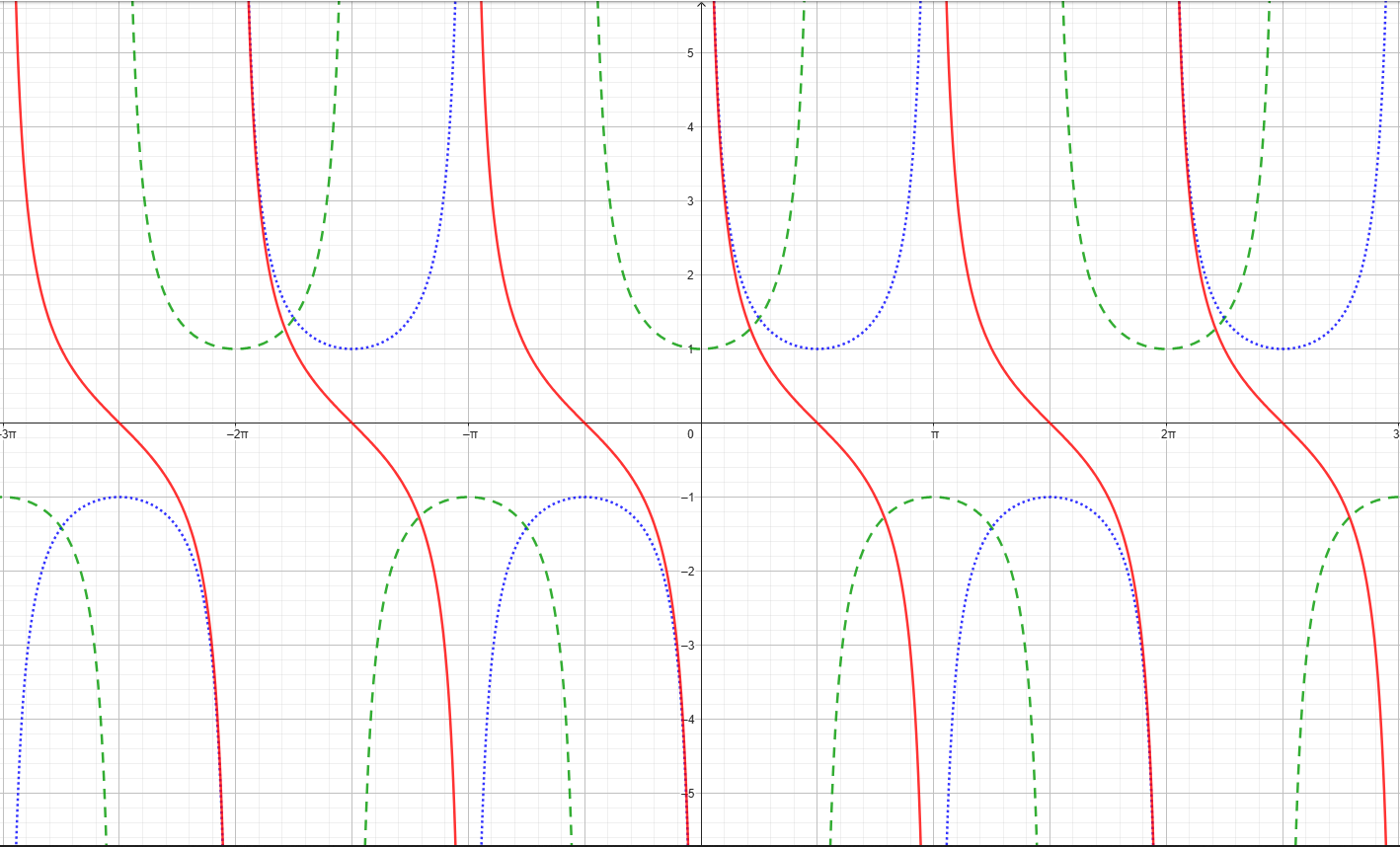
Further trig functions: There are three more trig functions that you should be aware of. Again, these are not independent trig functions but are one over the familiar trig functions. These are:
\(\seteqnumber{0}{2.}{0}\)\begin{align*} \sec x &=\frac {1}{\cos x},\\ \csc x &=\frac {1}{\sin x},\\ \cot x &=\frac {1}{\tan x}. \end{align*} Plots of these three functions are shown in fig. 2.8.
2.3 Logarithms and Exponentials
Another pair of very useful functions which we need to be familiar with are the logarithm and the exponential function.
In your previous maths courses you may have come across the fact that we call powers exponents, e.g. in an expression \(f(x)=x^{b}\) then \(b\) is called the exponent„ or the index. An exponential function is then a function like
\(\seteqnumber{0}{2.}{0}\)\begin{equation*} f(x)=b^{x}, \end{equation*}
where a constant5 \(b\) is raised to the power of the variable \(x\). In this case the number \(b\) is called the Base of the exponential function.
The exponential function with base \(2\) is shown in fig. 2.9. It turns out that by appropriate scaling of \(x\) different bases are related6 so we only need one standard basis.
When working with binary the basis \(b=2\) is chosen, while in scientific notation \(b=10\) is chosen. Nowadays the basis in general use is denoted \(e\) or \(\exp \) with \(\exp (x)\) called the exponential function.
5 here \(b>0\) and \(b\neq 1\).
6 To get an idea of this consider that \(2^{x}=4^{x/2}\) so we can always transform from base \(2\) into base \(4\). In general we need to use the logarithm function that we will meet shortly.
-
Mathematical Diversion 2.3. Warning! When talking to mathematicians there is a difference between \(e\) and \(\exp \), the first one is a number, close to \(2.71828\dots \), while \(\exp \) is a function. Often we will use \(e^{x}\) and \(\exp (x)\) interchangeably, but occasionally it is important to know the difference. The main difference is that \(\exp (x)\) is a one-to-one function, in particular when \(x=1/2\) we have that \(\exp (1/2)\simeq 1.65\) while when taking \(\sqrt {e}=e^{1/2}\) we need to pick either the positive or negative square root. Most likely you can just forget this distinction and work with \(e^{x}\) and \(\exp (x)\) as if they were the same thing. However, it is worth seeing the distinction at least once.

The reason for picking \(e\) as the basis is that simplifies some of the algebra associated with exponential functions, it also has the advantage that the tangent to the curve has gradient \(1\) at \(x=0\). This last part boils down to
\(\seteqnumber{0}{2.}{0}\)\begin{equation} e\simeq \left (1+h\right )^{\frac {1}{h}} \label {eq: exp approximation} \end{equation}
for \(h\) close to zero.

Closely related to \(\exp \) is its inverse function, called the logarithm function. You will see it written as either \(\log (x)\) or \(\ln (x)\), or rarely as \(\log _{e}(x)\) where the base is made explicit.
As this is an inverse function it is defined as the solution to the equation \(e^{y}=x\). For example \(e^{y}=4\) is solved by \(y=\ln (4)\).
The graphs of both \(\exp (x)\) and \(\ln (x)\) are shown in fig. 2.10. Note that we are, currently, not defining \(\ln \) when \(x\) is negative 7. You may have guessed that we could take a logarithm in a different basis since it is defined so that
\(\seteqnumber{0}{2.}{1}\)\begin{equation*} \ln (\exp (x))=x=\exp (\ln (x)). \end{equation*}
This is why there are several slightly different ways of writing the logarithm. If you learnt about it in school you probably used \(\log (x)\) to mean log with base \(10\). In this module if we work with a basis other than \(e\) we will make this explicit by writing \(\log
_{b}(x)\) to mean log with base \(b\).
To be clear \(\log _{b}(x)\) is the function defined such that
\(\seteqnumber{0}{2.}{1}\)\begin{equation*} \log _{b}(b^{x})=x=b^{\log _{b}(x)}. \end{equation*}
A nice property of exponentials and logarithms is that they map addition to multiplication. What this means is that
\(\seteqnumber{0}{2.}{1}\)\begin{align*} \exp (a)\exp (b)&=\exp (a+b),\\ \ln (ab)&=\ln (a)+\ln (b),\\ \ln \left (\frac {a}{b}\right )&=\ln (a)-\ln (b). \end{align*}
Some of the other properties of these functions are that:
\(\seteqnumber{0}{2.}{1}\)
\begin{align*}
\exp (-x)&=\frac {1}{\exp (x)},\\ \exp (x)&>0,\\ \exp (x)&\to \infty \quad \text {as } x\to \infty ,\\ \exp (x)&\to 0 \quad \text {as } x\to -\infty ,\\ \ln (x) &\to \infty \quad \text {as } x\to \infty ,\\ \ln
(x)&\to -\infty \quad \text {as } x\to 0^{+}.
\end{align*}
We will return to discussing limits shortly, but here the statement \(\exp (x)\to \infty \) as \(x\to \infty \) means that the function \(\exp (x)\) becomes infinitely large as \(x\) becomes infinitely large. The terminology for this is that \(\exp (x)\)
diverges as \(x\) tends to infinity.
The final, useful, identity about logarithms is how to change the basis. The change of basis formula is
\(\seteqnumber{0}{2.}{1}\)\begin{equation} \log _{b}(x)=\frac {\log _{a}(x)}{\log _{a}(b)}. \label {eq:log change of base} \end{equation}
As with trig functions in section 2.2, \(\ln \) and \(\exp \) are useful when solving equations. There are lots of examples in [Dawkins, 2025b] but we will go through a couple of examples here, there will be more on the tutorial sheets.
7 If you study more mathematics you will discover that we can make sense of \(\ln (x)\) when \(x\) is negative. However, it is no longer real and we need to understand complex numbers to make sense of it.
-
Example 2.6. Consider the equation
\(\seteqnumber{0}{2.}{2}\)\begin{equation*} x e^{-x} -x =0. \end{equation*}
The first step in solving this is to factor out the \(x\) common to both terms. Note that we cannot divide by \(x\) as at this stage we do not know if it will be zero. This gives us
\(\seteqnumber{0}{2.}{2}\)\begin{align*} x e^{-x} -x &=0\\ x\left (e^{-x}-1\right )&=0, \end{align*} so we get two possibilities8: either \(x=0\) or \(e^{-x}-1=0\). If we had divided by \(x\) we would have missed that \(x=0\) is a solution, and would not have completely solved the problem. Consider the second case,
\(\seteqnumber{0}{2.}{2}\)\begin{align*} e^{-x}&=1\\ -x&=\ln (1)=0 \end{align*} so this other case also reduces to \(x=0\) and we only have one solution in this case.
-
Example 2.7. Consider the equation
\(\seteqnumber{0}{2.}{2}\)\begin{equation*} \frac {1}{2}\ln \left (x^{2}\right )-\ln \left (x-1\right )=4. \end{equation*}
If we make use of the log rules we have that \(\ln (x^{2})/2=\ln (\sqrt {x^{2}})=\ln x\), where we take the positive square root as currently we do not know how to make sense of logarithms with negative arguments. The equation thus becomes
\(\seteqnumber{0}{2.}{2}\)\begin{align*} 4&=\frac {1}{2}\ln \left (x^{2}\right )-\ln \left (x-1\right )\\ &=\ln \left (x\right )-\ln \left (x-1\right )\\ &=\ln \left (\frac {x}{x-1}\right ). \end{align*} Now we can exponentiate both sides and rearrange to solve for \(x\):
\(\seteqnumber{0}{2.}{2}\)\begin{align*} \frac {x}{x-1}&=e^{4}\\ x&=e^{4}\left (x-1\right )\\ x&=-e^{4}+xe^{4}\\ x\left (1-e^{4}\right )&=-e^{4}\\ x&=-\frac {e^{4}}{1-e^{4}}=1.01866. \end{align*}
When we get an answer like this we need to check that it does not give a negative argument in any of the original logarithms, here we are fine since both \(x^{2}\) and \(x-1\) are positive.
It may seem like example 2.7 took quite a bit of working out, but with practice you will get faster at solving problems like this. In the lectures you will frequently hear me paraphrasing George Pólya and saying that Mathematics is not a spectator sport. This means that while reading these notes and attending the lectures can help you in your learning there is no substitute for actually rolling your sleeves up and solving problems. Remember that most modules expect you to be putting in around three hours of self study for every hour of contact time.
2.4 Hyperbolic functions
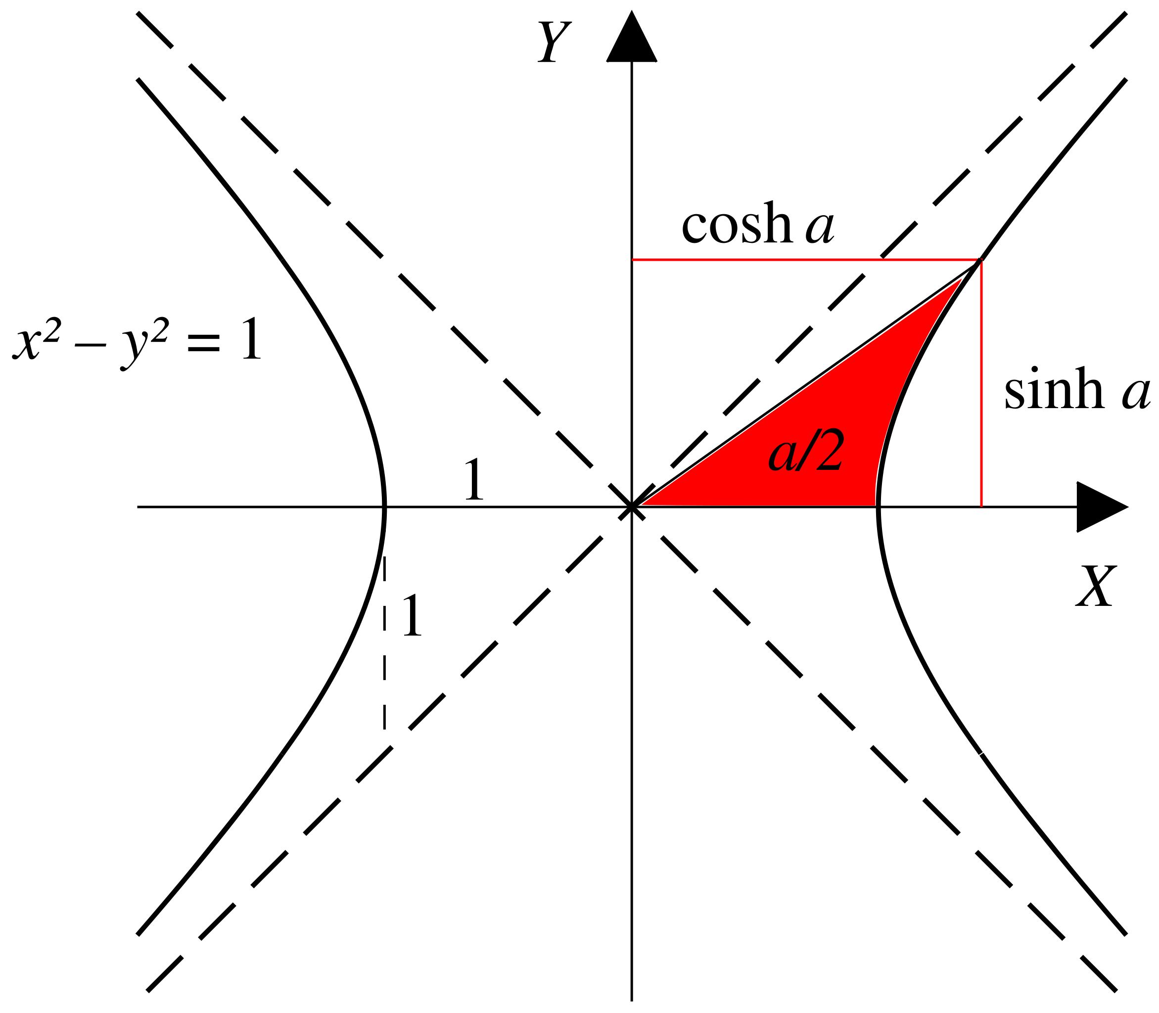
The next class of functions that it is useful to know about are the hyperbolic trig functions. As shown in fig. 2.11, the hyperbolic trig functions are the analogue of the standard trig functions
of section 2.2 but adapted to the geometry of the hyperbola, \(x^{2}-y^{2}=1\) rather than the circle \(x^{2}+y^{2}=1\). For the standard trig functions, their argument was an angle related to how far round the
unit circle we had gone. In the hyperbolic case the angle is now twice the shaded area shown in section 2.2.
There is a hyperbolic equivalent of all of the standard trig functions, and the notation is very similar just with an added \(h\) at the end:
-
• hyperbolic sine \(\sinh \),
-
• hyperbolic cosine \(\cosh \),
-
• hyperbolic tangent \(\tanh \),
-
• inverse hyperbolic sine \(\arcsinh \),
-
• inverse hyperbolic cosine \(\arccosh \),
-
• inverse hyperbolic tangent \(\arctan \).
There are also hyperbolic versions of the other trig functions but we will not be as concerned with them here.
As in the regular trig case the hyperbolic tangent is defined in terms of the other two functions as
\(\seteqnumber{0}{2.}{2}\)\begin{equation} \tanh (x)=\frac {\sinh (x)}{\cosh (x)}. \label {eq: hyperbolic tangent} \end{equation}
The hyperbolic trig functions are actually defined in terms of the odd and even parts of the exponential function9 as follows:
\(\seteqnumber{0}{2.}{3}\)\begin{align} \sinh (x)&=\frac {e^{x}-e^{-x}}{2}, \label {eq: sinh exp}\\ \cosh (x)&=\frac {e^{x}+e^{-x}}{2}. \label {eq: cosh exp} \end{align} They have the following useful properties:
\(\seteqnumber{0}{2.}{5}\)
\begin{align*}
\sinh (-x)&=-\sinh (x),\\ \cosh (-x)&=\cosh (x),\\ \cosh ^{2}(x)-\sinh ^{2}(x)&=1,\\ 1-\tanh ^{2}(x)&=\sech ^{2}(x).
\end{align*}
These are very similar to the identities satisfied by the ordinary trig functions. However, the sign in front of \(\sinh (x)\) and \(\tanh (x)\) is negative while that in front of \(\sin (x)\) and \(\tan (x)\) in the equivalent formulae was positive. The rule of thumb
when converting from identities for trig functions to identities for hyperbolic trig functions is to send \(\cos ^{2}(x)\to \cosh ^{2}(x)\) and \(\sin ^{2}(x)\to -\sinh ^{2}(x)\). There are also analogues of the addition of angle identity formulas that you can try to
derive if you are interested.
9 If you have come across complex numbers then you may know that this is only true for real \(x\), if the argument is imaginary then relationships like this hold between the exponential function and the standard trig functions. We may see this in the advanced topics section of the module if there is enough time.
-
Example 2.8. Consider the hyperbolic equation \(\cosh (x)-5\sinh (x)-5=0\) from chapter 3.7 in [Riley et al., 2006]. The easiest way to solve this is to use the definitions of the hyperbolic functions in terms of the exponential function. This transforms the equation into
\(\seteqnumber{0}{2.}{5}\)\begin{equation*} \frac {1}{2}\left (e^{x}+e^{-x}\right )-\frac {5}{2}\left (e^{x}-e^{-x}\right )-5=0, \end{equation*}
which we rearrange to give
\(\seteqnumber{0}{2.}{5}\)\begin{equation*} 0=e^{x}\left (\frac {1}{2}-\frac {5}{2}\right )+e^{-x}\left (\frac {1}{2}+\frac {5}{2}\right )-5=-2e^{x}+3e^{-x}-5. \end{equation*}
Then multiply through by \(-e^{x}\), which is allowed since this is never zero, to get
\(\seteqnumber{0}{2.}{5}\)\begin{equation*} 2e^{2x}+5e^{x}-3=0. \end{equation*}
Now we could either let \(y=e^{x}\) and use the quadratic formula to solve for \(y\) or we can factorise this to get
\(\seteqnumber{0}{2.}{5}\)\begin{equation*} \left (2e^{x}-1\right )\left (e^{x}+3\right )=0, \end{equation*}
so there are two solutions: \(e^{x}=1/2\) or \(x=-\ln (2)\), and \(e^{x}=-3\) or \(x=\ln (-3)\). Remember we have not discussed how to make sense of the logarithm of a negative number so for us there is only one real solution, \(x=-\ln (2)\).
Since the hyperbolic trig functions are related to the exponential function you can probably guess that their inverses are related to the logarithm. It is worth thinking about how to show this relationship. I will show you how to do this for \(\sinh (x)\) and \(\tanh (x)\) but leave deriving the identify for \(\cosh (x)\) as an exercise for the interested reader.
-
Example 2.9. Consider \(y=\arcsinh (x)\), we can invert this to give \(x=\sinh (y)\). Next if we make use of eqs. (2.4) and (2.5) we have that
\(\seteqnumber{0}{2.}{5}\)\begin{align*} e^{y} &=\cosh (y)+\sinh (y)\\ &=\sqrt {1+\sinh ^{2}(y)}+\sinh (y)\\ &=\sqrt {1+x^{2}}+x. \end{align*} Taking \(\ln \) of both sides then gives that
\(\seteqnumber{0}{2.}{5}\)\begin{equation} \arcsinh (x)=y=\ln \left (\sqrt {1+x^{2}}+x\right ). \label {eq: arcsinh log} \end{equation}
If you do a similar calculation for \(y=\arccosh (x)\) you will find that
\(\seteqnumber{0}{2.}{6}\)\begin{equation} \arccosh (x)=\ln \left (x\pm \sqrt {x^{2}-1}\right ). \label {eq: arccosh log} \end{equation}
You should think about why there is a \(\pm \) in this formula but there was not one in eq. (2.6).
-
Example 2.10. Consider \(y=\arctanh (x)\), which inverts to \(x=\tanh (y)\). Using the definition of \(\tanh (y)\) as being \(\sinh (y)/\cosh (y)\) and eqs. (2.4) and (2.5) we have that
\(\seteqnumber{0}{2.}{7}\)\begin{equation*} x=\frac {e^{y}-e^{-y}}{e^{y}+e^{-y}} \end{equation*}
which is equivalent to
\(\seteqnumber{0}{2.}{7}\)\begin{equation*} \left (x+1\right )e^{-y}=\left (1-x\right )e^{y}. \end{equation*}
which can be further rearranged to give
\(\seteqnumber{0}{2.}{7}\)\begin{align*} e^{2y}&=\frac {1+x}{1-x},\\ \Rightarrow e^{y}&=\sqrt {\frac {1+x}{1-x}},\\ y&=\ln \left (\sqrt {\frac {1+x}{1-x}}\right ). \end{align*} This gives that
\(\seteqnumber{0}{2.}{7}\)\begin{equation} \arctanh (x)=\frac {1}{2}\ln \left (\frac {1+x}{1-x}\right ). \label {eq: arctanh log} \end{equation}
You may be asking why we have spend the time deriving these identities for the hyperbolic functions, and why we discussed their relationship with the exponential function. This is because when we start to differentiate or integrate hyperbolic functions it is often more straightforward to use the expressions involving exponentials and logarithms.
2.5 Limits and asymptotics
We have now spent quite a bit of time discussing different examples of functions and their properties, as well as how to plot them. If we consider the plot of the tangent function in fig. 2.7 you may have asked at
the time, what happens when the red line goes off the top of the page and reappear at the bottom? If we followed both lines we would see that they are getting closer and closer to the point \(x=\uppi /2\). This idea of zooming in on a particular value \(x=a\) and asking
what happens to a function there is known as taking a limit as \(x\) approaches \(a\) and is denoted \(\lim _{x\to a}f(x)\).
If the function is well behaved at the point \(a\), then the limit is just the value of the function evaluated at \(a\), \(f(a)\). For example
\(\seteqnumber{0}{2.}{8}\)\begin{equation*} \lim _{x\to 0}\cos (x)=1=\cos (0). \end{equation*}
The value of the limit does not have to be finite, it can head off to infinity. A good example of this is the exponential function which just keeps getting larger as \(x\) increases. We denote this by
\(\seteqnumber{0}{2.}{8}\)\begin{equation*} \lim _{x\to \infty }\exp (x)\to \infty . \end{equation*}
Notice that since the value of the limit is infinite we do not write an equals sign but instead use \(\to \) to denote that the limit diverges10. There are lots of other examples of functions that diverge, and not always for large \(x\). A nice example to
have in mind is \(y=1/x^{2}\) which diverges as \(x\to 0\).
In the case of \(\tan (x)\) we can observe that \(\lim _{x\to \uppi /2}\tan (x)\) will take on different values depending on if \(x\) is approaching \(\uppi /2\) from above or below. This means that the limit does not exist. In section 2.6 we will discuss the consequences of this for the function in more detail. If we are taking the limit from above we often say \(x\to a^{+}\), while the limit from below is denoted \(x\to a^{-}\). In this case
\(\seteqnumber{0}{2.}{8}\)\begin{align*} \lim _{x\to \frac {\uppi }{2}^{+}}\tan (x)&\to \infty ,\\ \lim _{x\to \frac {\uppi }{2}^{-}}\tan (x)&\to -\infty , \end{align*} so \(\tan (x)\) diverges in different directions depending on how we approach \(\uppi /2\).
-
Mathematical Diversion 2.4. Putting our mathematician’s hats on for a brief moment, we would say that limit of a function \(f(x)\) as \(x\) approaches \(a\) is \(L\) and write it as
\(\seteqnumber{0}{2.}{8}\)\begin{equation*} \lim _{x\to a}f(x)=L, \end{equation*}
as long as we can make \(f(x)\) as close to \(L\) as we want for all \(x\) sufficiently close to \(a\) on both sides, without taking \(x=a\).
If this was a maths module we would be even more precise and give what is called an \(\upepsilon ,\updelta \) definition. Fortunately for all of us this is not a maths module and we can focus on a more practical/ working definition rather than getting bogged down in the abstract details. If you are interested to know how to do this in detail, the section “The Definition of a Limit” in [Dawkins, 2025b] is a good place to look.
Remember that \(x\to a\) does not mean that \(x\) becomes equal to \(a\), it just means that \(x\) is getting close to \(a\). It is also possible that \(f(x)\) may never equal \(L\), but also just get close to it. This is especially true when we take the limit near a point that the function is not defined at, e.g. \(x\to \uppi /2\) for \(\tan (x)\).
Curve sketching is a useful way to understand the main features of a function and can help us to know if the limit exists and if we have the same limit when approaching from different directions.
-
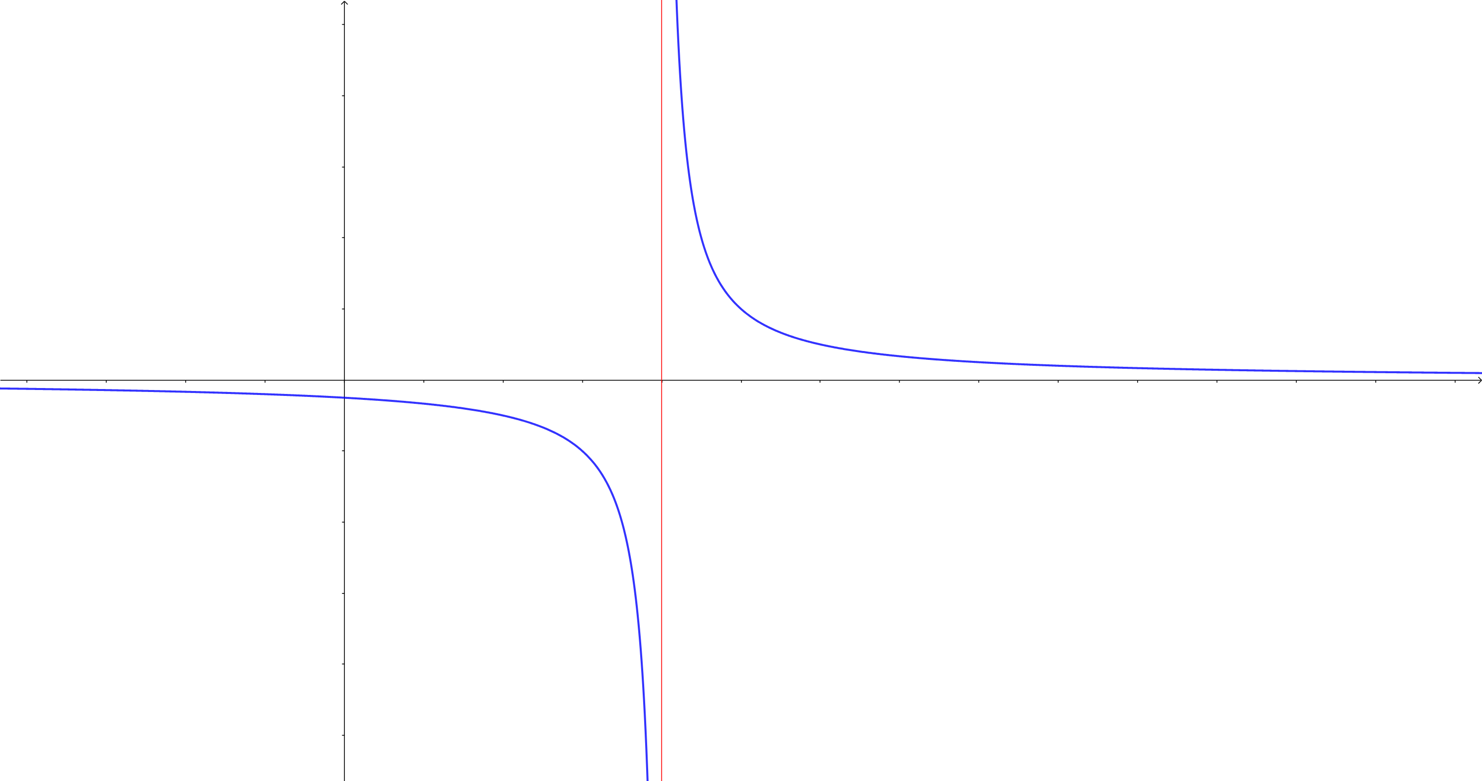
Example 2.11. Consider the function
\(\seteqnumber{0}{2.}{8}\)\begin{equation} f(x)=\frac {1}{x-2}, \label {eq: reciprocal of x-2} \end{equation}
defined for \(x\neq 2\).
Notices that for \(x\to \pm \infty \) \(f(x)\to 0\), in fig. 2.12 we see that the plot approaches the horizontal axis asymptotically11. We can also observe that for \(a\neq 2\) \(f(x)\to f(a)\) for \(x\to a\). The only point where we need to be careful is when \(x\) tends to \(2\) looking at fig. 2.12 we see that if we approach \(2\) from above that \(f(x)\to \infty \) while if we approach \(2\) from below \(f(x)\to -\infty \).
Note that the fact that \(f(x)\) is not defined at \(x=2\) has no bearing on the limiting behaviour.
The general rule when curve sketching is to set \(y=f(x)\) for the function of interest \(f(x)\), and then to investigate the following:
-
• The intercepts of \(f(x)\), these are the points where the function meets or crosses the coordinate axes, e.g. \(f(x=0)\) and \(f(x)=0\), as these position the graph relative to the coordinate axes.
-
• What happens to \(y\) as \(x\to \pm \infty \)?
-
• Which values of \(x\) make \(y\to \pm \infty \)?
-
• Does the function have any symmetry? For example does \(f(-x)=f(x)\) (\(f\) is even), or \(f(-x)=-f(x)\) (\(f\) is odd).
-
• Is the function periodic?
Note that a function can have several of these interesting features. e.g. the trig functions are all periodic, while \(\sin (x)\) and \(\tan (x)\) are odd functions and \(\cos (x)\) is an even function.
-
Mathematical Diversion 2.5. An asymptote to a curve is a straight line that becomes close to the curve as either \(x\) or \(y\) tend to \(\pm \infty \). In our above example the curve of eq. (2.9) has two asymptotes, the horizontal \(x\)-axis for \(x\to \pm \infty \) and the vertical line \(x=2\) for \(x\to 2\).
When sketching a curve it is often useful to start by drawing the asymptotes in as they help you to know how the function will behave in certain regions of the plot. In some books you may see \(f(x)\asymp mx +c\) as \(x\to \infty \) to signify that the straight line \(y=mx+c\) is an asymptote to the graph of \(f(x)\) as \(x\) tends to infinity.
-
Example 2.13. Consider the rational function
\(\seteqnumber{0}{2.}{9}\)\begin{equation*} f(x)=\frac {x^{2}+4x-12}{x^{2}-2x} \end{equation*}
and compute its limit as \(x\to 2\).
Looking at the function you may think that it will diverge as \(x\to 2\) since the denominator vanishes there. However the first step is always to look at if there are any common factors between the numerator and denominator. Factorising both we have
\(\seteqnumber{0}{2.}{9}\)\begin{align*} f(x)&=\frac {x^{2}+4x-12}{x^{2}-2x}\\ &=\frac {(x+6)(x-2)}{x(x-2)}\\ &=\frac {x+6}{x}. \end{align*} So the denominator does not vanish at \(x=2\). We can now evaluate the limit to be
\(\seteqnumber{0}{2.}{9}\)\begin{equation*} \lim _{x\to 2}f(x)=\lim _{x\to 2}\frac {x+6}{x}=\frac {8}{2}=4. \end{equation*}
The limit is the same regardless of which direction we approach \(2\) from.
As a warning, this approach of tabulating the values does not work if the function is oscillating. For example, if you try to evaluate the limit as \(x\to 0\) of \(\cos \left (\uppi /x\right )\) it can look like it is tending to a constant if we are not careful with the values that we pick. However, if we plot the function we see that it is highly oscillatory around zero.
-
Example 2.15. Consider the rational function
\(\seteqnumber{0}{2.}{9}\)\begin{equation*} f(x)=\frac {x^{3}+x^{2}-5x-2}{2x^{3}-7x^{2}+4x+4}. \end{equation*}
It has three interesting limits, \(x\to 0,\infty ,2\). We can evaluate the first two of these here, but need to leave the third, \(x\to 2\) until we have learnt about L’Hôpital’s rule in chapter 8. We will do \(x\to 0\) first. As usual we check that the numerator and denominator both make sense as \(x\to 0\) and then can evaluate the limit
\(\seteqnumber{0}{2.}{9}\)\begin{align*} \lim _{x\to 0}f(x)&=\lim _{x\to 0}\frac {x^{3}+x^{2}-5x-2}{2x^{3}-7x^{2}+4x+4}\\ &=\frac {-2}{4}\\ &=-\frac {1}{2}. \end{align*}
Next we do the \(x\to \infty \) limit. Before we do this we need to multiply \(f(x)\) by \(x^{-3}/x^{-3}\) so that it becomes
\(\seteqnumber{0}{2.}{9}\)\begin{align*} \lim _{x\to \infty }f(x) &=\lim _{x\to \infty }\left (\frac {x^{-3}}{x^{-3}}\frac {x^{3}+x^{2}-5x-2}{2x^{3}-7x^{2}+4x+4}\right )\\ &=\lim _{x\to \infty }\left (\frac {1+x^{-1}-5x^{-2}-2x^{-3}}{2-7x^{-1}+4x^{-2}+4x^{-3}}\right )\\ &=\frac {1}{2}. \end{align*}
Remember that when evaluating a limit we want to look for as many cancellations as possible to simplify the calculation. This can be looking for common factors between the numerator and denominator, but can also mean fully expanding out all terms as there may be cancellations hidden by the way the function has been written.
Often it is useful to plot a function when we are estimating the limit, while this is not compulsory it can be very helpful, particularly if as in the case of \(\tan (x)\), the value of the limit depends on the direction of approach.
-
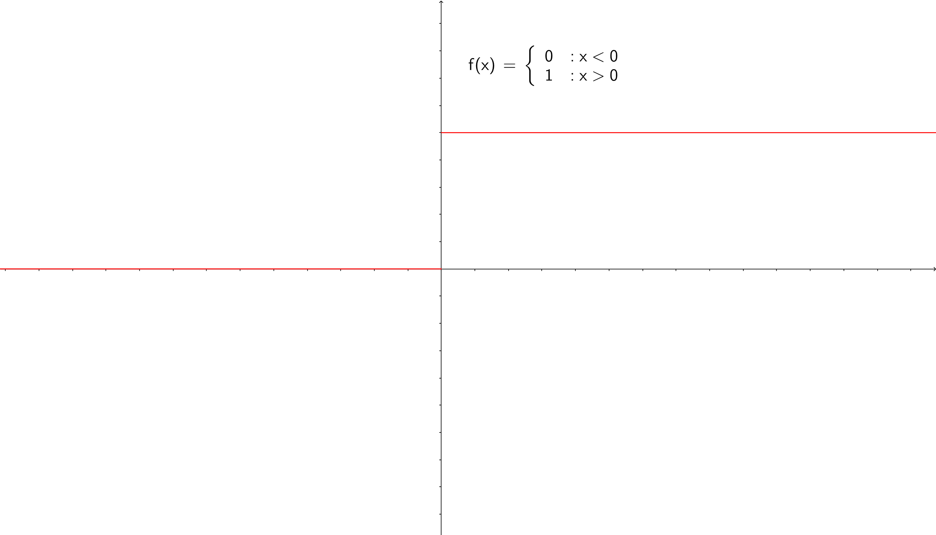
Example 2.16. Consider the step function
\(\seteqnumber{0}{2.}{9}\)\begin{equation} f(x)=\begin{cases} &0 \quad x < 0\\ &1 \quad x\geq 0, \end {cases} \label {eq: step function} \end{equation}
shown in fig. 2.13. By looking at the graph we see that the limit of \(f(x)\) as \(x\to 0\) will depend on the direction of approach. If we start from below zero it is clear that \(f(x)\to 0\), while starting above zero it is clear that \(f(x)\to 1\). In contrast to the case of \(\tan (x)\) the function is not diverging in the limit, but we still end up with a One Sided Limit12
-
Mathematical Diversion 2.6. Note that it can be dangerous to use \(\infty \) in calculations as if it were a number. This is because there are certain limits and other expressions that we may see which do not make sense:
\(\seteqnumber{0}{2.}{10}\)\begin{equation*} \infty ^{0}, \quad \infty -\infty , \quad \frac {0}{0}, \quad 0^{0}, \quad \frac {\infty }{\infty }, \quad \frac {\infty }{0}, \quad \frac {1}{0}. \end{equation*}
Just because we see one of these expressions coming out a limit does not necessarily mean that the limit does not exist. It can instead mean that we need to be very careful how we evaluate the limit. In chapter 8 we will discuss L’Hôpital’s rule which is a techniques for evaluating limits that initially look like they do not make sense.
There are a few limits that we need to know that we will not prove here, time permitting we will prove these in chapter 8, but you can also look at the “Proof of Trig Limits” section of Dawkins [2025b] to see one approach to proving them. These limits are
\(\seteqnumber{0}{2.}{10}\)\begin{align} \lim _{x\to 0}\frac {\sin x}{x}&=1, \label {eq: sin limit}\\ \lim _{x\to 0}\frac {\cos x -1}{x}&=0, \label {eq: cos limit}\\ \lim _{h\to 0}\frac {e^{h}-1}{h}&=1, \label {eq: exp limit}\\ \lim _{h\to 0}\frac {\ln (1+h)}{h}&=1. \label {eq: ln limit} \end{align} Note that eq. (2.13) is equivalent to eq. (2.1) which we discussed above as one of the definitions of the exponential function.
2.6 Continuity and differentiability
Now that we have some examples of functions and understand how to take limits, we can define two properties of a function which will be very important later in the course: continuity and differentiability.
A function \(f(x)\) is said to be continuous at a point \(x=a\) if
\(\seteqnumber{0}{2.}{14}\)\begin{equation} \lim _{x\to a}f(x)=f(a). \label {eq: continuity} \end{equation}
If \(X\) is the domain of \(f(x)\), we say that \(f\) is continuous on \(X\) if it is continuous at each point in \(X\), often we would just say that \(f\) is a continuous function. As a rule of thumb, we can say that a function is continuous if its graph can be drawn from
start to finish without taking your pen off the paper. Functions which are not continuous will have jumps or divergences at the point that fails to be continuous.
If we have a rational function then we can find where it is not continuous, called being discontinuous, by finding the roots of the denominator.
-
Mathematical Diversion 2.7. If we are being careful we need to give three parts to the definition of continuity:
-
1) The limit of \(f(x)\) as \(x\to a\) exists.
-
2) The value of \(f(x)\) is defined at \(x=a\). i.e. \(f(a)\) is defined and is finite.
-
3) The limit of \(f(x)\) as \(x\to a\) agrees with the value of \(f(a)\).
This is another place where as this is not a course for mathematicians we can combine all three of these into the one statement in eq. (2.15). This is another example of being able to use a working definition and not needing to get sidetracked by all of the technical details.
-
-
Example 2.17. We have already met several examples of continuous and discontinuous functions:
-
• The trig functions \(\cos (x)\) and \(\sin (x)\) are continuous on all of \(\R \).
-
• The exponential function \(\exp (x)\) is continuous on all of \(\R \).
-
• The natural logarithm is continuous on the positive real numbers \(\R \) as, currently we have not defined it for negative \(x\), and it diverges in the limit \(x\to 0\).
-
• The tangent function \(\tan (x)\) are not continuous on \(\R \) due to its divergences at \(\pm \frac {\uppi }{2},\pm \frac {3\uppi }{2},\dots {}\). However, it is continuous on its domain13 \(\left (-\frac {\uppi }{2},\frac {\uppi }{2}\right )\)
-
• The step function of eq. (2.10) is not continuous at \(x=0\).
-
• The function in eq. (2.9) has a discontinuity at \(x=2\)
-
Related to continuity is differentiability. A function \(f(x)\) is differentiable at a point \(a\) if the limit
\(\seteqnumber{0}{2.}{16}\)\begin{equation*} \lim _{x\to a}\frac {f(x)-f(a)}{x-a} \end{equation*}
exists. We call this limit the derivative of the function at the point \(a\),
\(\seteqnumber{0}{2.}{16}\)\begin{equation} f'(a)=\lim _{x\to a}\frac {f(x)-f(a)}{x-a}, \label {eq: rate of change at a} \end{equation}
the notation \(\frac {\ud f}{\ud x}(a)\) is sometimes used instead of \(f'(a)\). A function is called continuously differentiable if its derivative is also continuous.
It is important to note that differentiability at \(a\) implies continuity at \(a\), but continuity does not imply differentiability. For example the absolute value function shown in fig. 2.14 is continuous everywhere, but is only differentiable everywhere except at \(x=0\).

-
Example 2.19. Consider the modulus or absolute value function shown in fig. 2.14. We have said that this is a continuous function which is not differentiable at \(x=0\), but how do we show this? We do it by checking all of the limits.
Checking continuity at \(x=0\) is left as an exercise. For differentiability we need to check the limits as \(x\to 0^{+}\) and \(x\to 0^{-}\).
In the first one we have:
\(\seteqnumber{0}{2.}{17}\)\begin{equation*} \lim _{x\to 0^{+}}\frac {f(x)-f(0)}{x}=\lim _{x\to 0^{+}}\frac {x-0}{x}\lim _{x\to 0^{+}}1=1, \end{equation*}
while approaching from the other direction gives:
\(\seteqnumber{0}{2.}{17}\)\begin{equation*} \lim _{x\to 0^{-}}\frac {f(x)-f(0)}{x}=\lim _{x\to 0^{-}}\frac {(-x)-0}{x}\lim _{x\to 0^{-}}-1=-1. \end{equation*}
These do not agree, so the limit does not exist and the modulus function is not differentiable.

The fraction in eq. (2.17) may look familiar to you. If we had a straight line \(y=f(x)=mx+c\) where \(m\) is the gradient of the straight line and \(c\) is the \(y\)-intercept, then calculating this fraction gives
\(\seteqnumber{0}{2.}{17}\)\begin{equation*} \frac {f(x)-f(a)}{x-a}=\frac {mx+c-(ma+c)}{x-a}=\frac {m(x-a)}{x-a}=m, \end{equation*}
which is the gradient of the curve. For a function that is not a straight line, this procedure gives the gradient of the straight line between \(x\) and \(a\). In the limit that \(x\to a\) this fraction becomes the gradient of the tangent line14 to the curve at \(a\). See fig. 2.16 for the example of the tangent to parabola \(y=x^{2}\).
-
Mathematical Diversion 2.8. The fraction
\(\seteqnumber{0}{2.}{17}\)\begin{equation*} \frac {f(x)-f(a)}{x-a} \end{equation*}
is sometimes referred to as the Newton quotient of the function \(f(x)\) at the point \(a\). This is after Isaac Newton because when calculating a derivative we are calculating this quotient for smaller and smaller differences \(x-a\).
